Panel Data and Fixed Effects in R

Claudius Gräbner-Radkowitsch

Panel Data and Fixed Effects in R

R

regression

statistics

causal-inference

tutorial

MA

Understand the logic of panel data, learn to distinguish within- from between-unit variation, estimate fixed effects models with fixest, and connect the FE identification argument to causal reasoning.

Author

Claudius Gräbner-Radkowitsch

Published

June 16, 2026

Modified

June 16, 2026

1 Introduction

Cross-sectional regression can tell us that richer countries are happier than poorer ones. But this comparison confounds income with every other stable characteristic that distinguishes rich countries from poor ones — culture, institutions, history, geography. Panel data — observations on the same units at multiple points in time — allow us to separate these stable background differences from the variation we actually care about.

Fixed effects (FE) estimation exploits the within-unit variation: when a country’s income rises above its own historical average, does its happiness rise too? By asking this question for each unit separately and averaging, FE eliminates all stable unit-level characteristics as potential confounders — observed or unobserved.

1.1 Research question

Does rising income make countries happier — and what would it take to interpret that relationship causally?

This question has a clear cross-sectional answer (yes, richer countries are happier) but a much less clear within-country answer — the Easterlin paradox. Panel methods let us be precise about which comparison we are making.

1.2 Data and packages

We use a country-level panel merging three sources: the World Happiness Report, World Bank WDI, and SWIID.

Getting the data

happiness_income.csv is a composite dataset prepared for this tutorial, merging the World Happiness Report, World Bank WDI, and SWIID. It is co-located with this resource at resources/r-programming/data/happiness_income.csv in the Method and Inquiry repository. Place it in a data/ subfolder next to this file before running the code.

Code

library(tidyverse)
library(fixest)
library(modelsummary)
library(flextable)
library(patchwork)

Code

dat <- read_csv("data/happiness_income.csv", show_col_types = FALSE) |>
  filter(!is.na(happiness), !is.na(GDP_pc))

glimpse(dat)

Rows: 1,729
Columns: 10
$ country      <chr> "Afghanistan", "Afghanistan", "Afghanistan", "Afghanistan…
$ iso2c        <chr> "AF", "AF", "AF", "AF", "AF", "AF", "AF", "AF", "AF", "AF…
$ iso3c        <chr> "AFG", "AFG", "AFG", "AFG", "AFG", "AFG", "AFG", "AFG", "…
$ year         <dbl> 2011, 2012, 2014, 2015, 2016, 2017, 2018, 2019, 2020, 202…
$ GDP_ppp      <dbl> 80913174278, 91231454558, 98965950295, 100402257641, 1026…
$ population   <dbl> 29347708, 30560034, 32792523, 33831764, 34700612, 3568893…
$ unemployment <dbl> 7.830, 7.875, 7.915, 9.032, 10.116, 11.184, 11.192, 11.18…
$ GDP_pc       <dbl> 2757.053, 2985.319, 3017.943, 2967.692, 2958.785, 2952.99…
$ happiness    <dbl> 4.2580, 4.0400, 3.5750, 3.3600, 3.7940, 3.6320, 3.2030, 2…
$ gini_disp    <dbl> 31.7, 31.8, 31.9, 31.9, 31.9, 31.9, NA, NA, NA, NA, NA, N…

Variable	Source	Description
`happiness`	World Happiness Report 2026	Life satisfaction (0–10, 3-year average)
`GDP_pc`	World Bank WDI	GDP per capita, PPP (constant 2017 int’l $)
`gini_disp`	SWIID 9.2	Disposable income Gini coefficient
`unemployment`	World Bank WDI	Unemployment rate (% of labour force)

2 Exploring the Data

2.1 Panel structure

Code

dat |>
  summarise(
    n_countries = n_distinct(country),
    n_years     = n_distinct(year),
    year_min    = min(year),
    year_max    = max(year),
    n_obs       = n()
  ) |>
  flextable() |> theme_vanilla() |> autofit()

n_countries	n_years	year_min	year_max	n_obs
144	13	2,011	2,024	1,729

The panel is unbalanced — not every country appears in every year. This is typical for survey-based cross-country data and causes no problems for fixed effects estimation.

2.2 The cross-sectional pattern

Code

dat |>
  group_by(country) |>
  summarise(
    happiness = mean(happiness, na.rm = TRUE),
    log_gdp   = mean(log(GDP_pc), na.rm = TRUE),
    .groups = "drop"
  ) |>
  filter(!is.na(happiness), !is.na(log_gdp)) |>
  ggplot(aes(log_gdp, happiness)) +
  geom_point(colour = "#2C5F8A", alpha = 0.7, size = 2) +
  geom_smooth(method = "lm", colour = "#D04A2F", se = TRUE,
              fill = "#D04A2F", alpha = 0.12, linewidth = 1) +
  labs(
    x = "Log GDP per capita (PPP), country mean",
    y = "Life satisfaction (0–10), country mean"
  ) +
  theme_minimal(base_size = 13)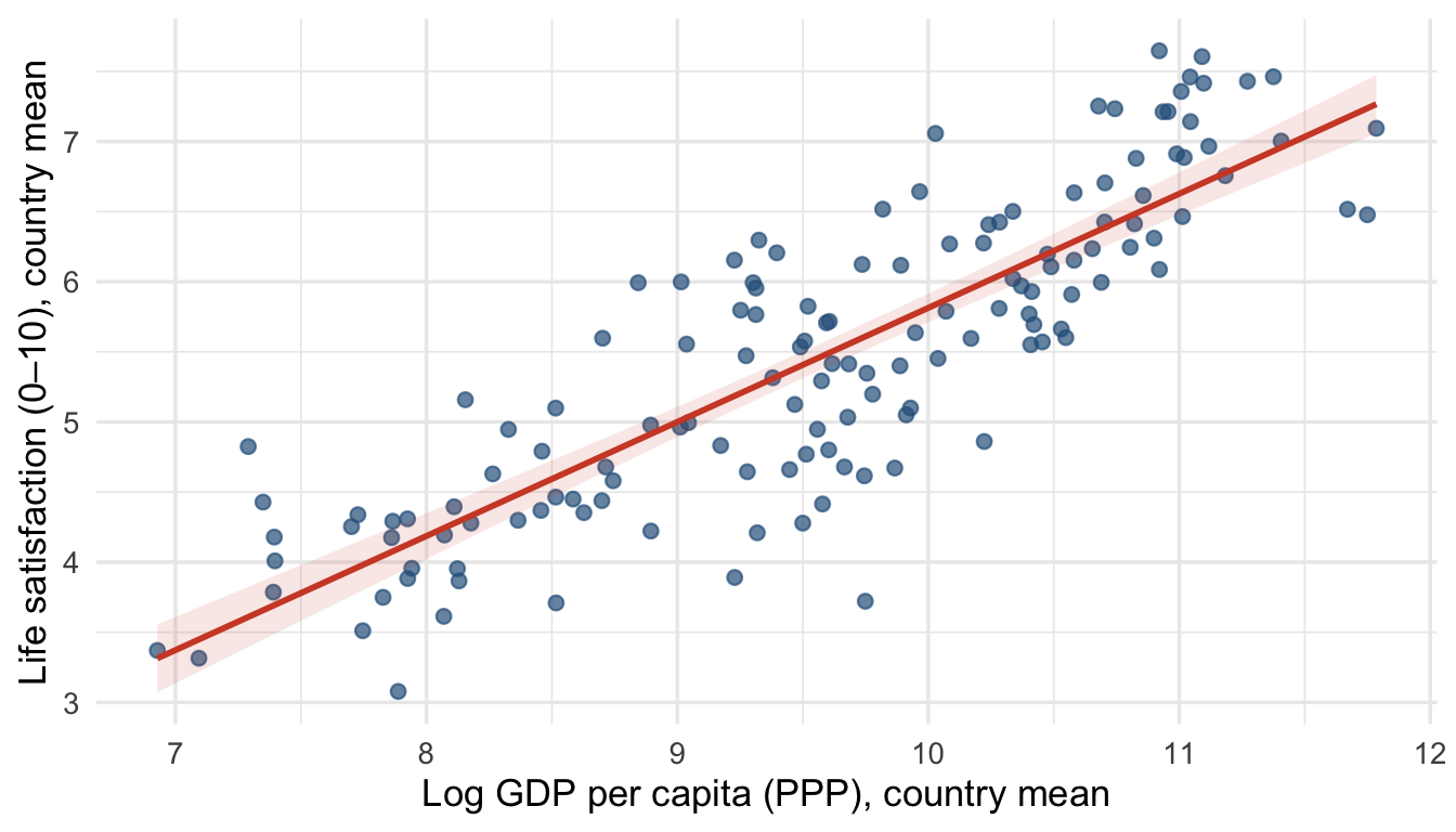

Figure 1: Average happiness and log GDP per capita by country (full-period means). Richer countries are clearly happier in cross-section.

The cross-sectional correlation is strong. But is this evidence that income causes happiness?

2.3 Within-country trends: the Easterlin challenge

Code

highlight <- c("United States", "Japan", "South Korea", "China", "Germany")

col_hl <- c(
  "United States" = "#D04A2F",
  "Japan"         = "#e67e22",
  "South Korea"   = "#8e44ad",
  "China"         = "#2C5F8A",
  "Germany"       = "#4A9B6F"
)

dat |>
  filter(country %in% highlight, !is.na(happiness)) |>
  ggplot(aes(year, happiness, colour = country)) +
  geom_line(linewidth = 1.1) +
  geom_point(size = 1.8) +
  scale_colour_manual(values = col_hl, name = NULL) +
  scale_x_continuous(breaks = seq(2006, 2024, by = 4)) +
  labs(x = NULL, y = "Life satisfaction (0–10)",
       caption = "Source: World Happiness Report (3-year averages)") +
  theme_minimal(base_size = 13)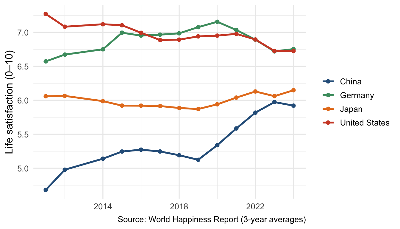

Figure 2: Happiness over time for selected countries. GDP per capita rose in all of them — but happiness trends diverge.

China’s GDP per capita roughly quadrupled over this period. Its happiness score rose only modestly. The United States had strong aggregate growth — yet happiness has trended flat or downward. This is the Easterlin paradox in real data.

3 The Model Progression

3.1 Step 0 — Pooled OLS: the naive baseline

Pooled OLS ignores panel structure entirely:

Code

m0 <- feols(happiness ~ log(GDP_pc), data = dat)

The large positive coefficient reflects the strong cross-sectional pattern — but it conflates between-country differences (richer country = happier country) with within-country change (rising income → rising happiness).

3.2 Why pooled OLS is biased

The pooled OLS error $\epsilon_{it}$ has two components:

\[\epsilon_{it} = \eta_i + v_{it}\]

$\eta_i$: everything stable about country $i$ that we do not observe — culture, institutions, social trust
$v_{it}$: genuine year-to-year noise

If $\eta_i$ correlates with $\log(\text{GDP}_{it})$ — which it clearly does, since institutional quality produces both high income and high happiness — pooled OLS is biased. This is omitted variable bias with an unobservable variable.

3.3 Step 1 — Country fixed effects

Country FE eliminates $\eta_i$ by subtracting each country’s time-mean from every variable:

\[\tilde{y}_{it} = y_{it} - \bar{y}_i \qquad \tilde{x}_{it} = x_{it} - \bar{x}_i\]

Because $\eta_i - \bar{\eta}_i = 0$, the stable country component drops out entirely. The coefficient is now identified from within-country variation only.

In fixest, add fixed effects with |:

Code

m1 <- feols(happiness ~ log(GDP_pc) | country,
            vcov = ~country,
            data = dat)

Note

vcov = ~country clusters standard errors at the country level. For panel data, clustering at the unit level is standard practice — it accounts for the serial correlation of errors within units.

3.4 Step 2 — Two-way fixed effects

Country FE removes stable country differences. But what about shocks that hit all countries in the same year — a global recession, a pandemic? Two-way FE adds a year fixed effect:

\[y_{it} = \alpha_i + \gamma_t + \beta \log(\text{GDP}_{it}) + v_{it}\]

$\hat\beta$ is now identified from variation that is neither explained by which country nor which year:

Code

m2 <- feols(happiness ~ log(GDP_pc) | country + year,
            vcov = ~country,
            data = dat)

3.5 Visualising the within-transformation

To build intuition, let us manually demean data for selected countries:

Code

within_dat <- dat |>
  filter(country %in% highlight) |>
  group_by(country) |>
  mutate(
    happiness_dm = happiness   - mean(happiness,    na.rm = TRUE),
    log_gdp_dm   = log(GDP_pc) - mean(log(GDP_pc),  na.rm = TRUE)
  ) |>
  ungroup()

p_raw <- dat |>
  filter(country %in% highlight) |>
  ggplot(aes(log(GDP_pc), happiness)) +
  geom_point(colour = "grey70", alpha = 0.4, size = 1.5) +
  geom_smooth(method = "lm", colour = "#D04A2F", se = FALSE, linewidth = 0.8, linetype = "dashed") +
  geom_smooth(aes(colour = country), method = "lm", se = FALSE, linewidth = 1) +
  scale_colour_manual(values = col_hl, guide = "none") +
  labs(x = "Log GDP per capita", y = "Happiness", title = "Raw data") +
  theme_minimal(base_size = 11)

p_demeaned <- within_dat |>
  ggplot(aes(log_gdp_dm, happiness_dm)) +
  geom_point(aes(colour = country), alpha = 0.6, size = 1.5) +
  geom_smooth(method = "lm", colour = "#D04A2F", se = FALSE, linewidth = 1) +
  scale_colour_manual(values = col_hl, name = NULL) +
  labs(x = "Log GDP (demeaned)", y = "Happiness (demeaned)", title = "Demeaned (within)") +
  theme_minimal(base_size = 11) +
  theme(legend.position = "bottom")

p_raw + p_demeaned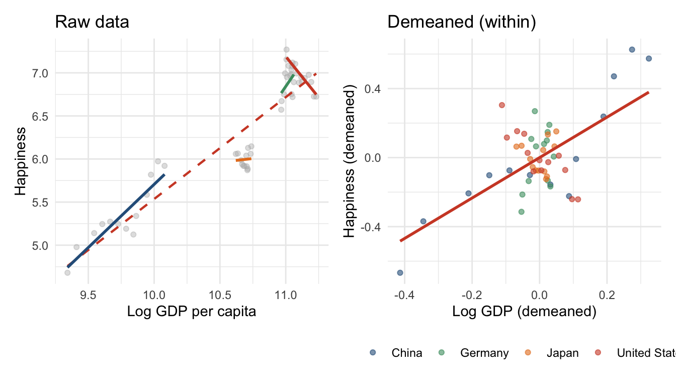

Figure 3: Raw data vs. demeaned data for selected countries. The between-country slope (dashed) is dominated by stable differences; within-country slopes (right panel) are what FE estimates.

The between-country slope (dashed, left) is steep. The within-country slope (right) is flatter — in some countries barely positive.

3.6 Side-by-side progression

Code

modelsummary(
  list("Pooled OLS" = m0, "Country FE" = m1, "Two-way FE" = m2),
  coef_map  = c("log(GDP_pc)" = "Log GDP per capita"),
  statistic = "conf.int", conf_level = 0.95,
  gof_map   = c("nobs", "r.squared", "r2.within"),
  stars     = TRUE,
  notes     = "95% CIs in brackets. Pooled OLS: HC1 SEs. FE models: clustered at country level.",
  output    = "flextable"
) |> autofit()

Table 1: Income and happiness: pooled OLS, country FE, and two-way FE. 95% confidence intervals in brackets. Within-R² is the relevant fit statistic for FE models.

	Pooled OLS	Country FE	Two-way FE
Log GDP per capita	0.813***	1.259***	1.554***
	[0.786, 0.840]	[0.829, 1.688]	[0.943, 2.164]
Num.Obs.	1729	1727	1727
R2	0.672	0.928	0.930
R2 Within		0.150	0.142
+ p < 0.1, * p < 0.05, p < 0.01, * p < 0.001
95% CIs in brackets. Pooled OLS: HC1 SEs. FE models: clustered at country level.

Reading the progression:

Pooled OLS → Country FE: The coefficient increases from 0.81 to 1.26. This is counterintuitive but real: the within-country income–happiness relationship is stronger than the cross-sectional comparison between countries. The cross-sectional estimate is compressed by diminishing returns at high income levels and by stable between-country happiness differences unrelated to income.
Country FE → Two-way FE: The coefficient increases further to 1.55. Year FE removes global shocks that simultaneously raised incomes and happiness everywhere; after removing those, the within-country signal is stronger.
Within-R²: income explains a meaningful but modest share of within-country happiness variation — happiness has many determinants beyond income.

4 Causal Interpretation

4.1 What FE controls for

Country FE already controls for all time-invariant country characteristics: stable institutions, culture, geography, social trust, historical development path. Year FE controls for global shocks in a given year.

What FE cannot control for: time-varying factors that change differently across countries and affect both income and happiness. Two obvious candidates: income inequality and unemployment.

Code

m3 <- feols(happiness ~ log(GDP_pc) + gini_disp + unemployment | country + year,
            vcov = ~country, data = dat)

4.2 What FE cannot fix

Limits of fixed effects

FE eliminates time-invariant confounders. It does not solve:

Time-varying confounders — variables that change within units and affect both income and happiness. Adding them explicitly (as gini_disp and unemployment above) is the right approach.
Reverse causality — happiness affecting income (harder to rule out with observational panel data)
Measurement error in the time-varying predictor — attenuation bias is amplified in FE estimation because the within-variation signal is smaller

The FE estimate should be understood as: “When a country’s income rises above its own historical average, controlling for global year shocks, does its happiness tend to rise?” — not as a clean causal effect.

5 Reporting Panel Results

Five rules for panel regression tables:

Show the progression — pooled OLS to your preferred specification
Report CIs, not SEs — statistic = "conf.int" in modelsummary
Report which FEs are included — in a table footnote, not as coefficient rows
Report the within-R² — r2.within in gof_map; the overall R² is inflated by the fixed effects
State the clustering level — always note it in the table footer

Code

modelsummary(
  list(
    "(1) Pooled OLS"      = m0,
    "(2) Country FE"      = m1,
    "(3) Two-way FE"      = m2,
    "(4) + Controls"      = m3
  ),
  coef_map  = c(
    "log(GDP_pc)"  = "Log GDP per capita",
    "gini_disp"    = "Gini coefficient",
    "unemployment" = "Unemployment rate"
  ),
  statistic = "conf.int", conf_level = 0.95,
  gof_map   = c("nobs", "r.squared", "r2.within"),
  stars     = TRUE,
  notes     = c(
    "95% CIs in brackets.",
    "Column (1): HC1 standard errors.",
    "Columns (2)–(4): clustered at country level.",
    "Country and year fixed effects in columns (3) and (4)."
  ),
  output = "flextable"
) |> autofit()

Table 2: Income and happiness: complete progression. Preferred specification: column (4).

	(1) Pooled OLS	(2) Country FE	(3) Two-way FE	(4) + Controls
Log GDP per capita	0.813***	1.259***	1.554***	1.376***
	[0.786, 0.840]	[0.829, 1.688]	[0.943, 2.164]	[0.666, 2.086]
Gini coefficient				-0.026
				[-0.059, 0.008]
Unemployment rate				-0.036***
				[-0.055, -0.017]
Num.Obs.	1729	1727	1727	1297
R2	0.672	0.928	0.930	0.945
R2 Within		0.150	0.142	0.194
+ p < 0.1, * p < 0.05, p < 0.01, * p < 0.001
95% CIs in brackets.
Column (1): HC1 standard errors.
Columns (2)–(4): clustered at country level.
Country and year fixed effects in columns (3) and (4).

6 Summary

Panel data tracks N units × T periods; within-unit variation is what fixed effects exploits
Pooled OLS conflates between- and within-unit variation and is biased when stable unit characteristics correlate with the predictor
Country FE (| country in feols) eliminates all time-invariant unit-level confounders
Two-way FE (| country + year) additionally removes year-specific global shocks
Cluster standard errors at the unit level to account for serial correlation
Within-R² is the correct fit statistic; overall R² is inflated by the fixed effects themselves

7 Further Reading

Békés, G. & Kézdi, G. (2021). Data Analysis for Business, Economics, and Policy. Ch. 24. gabors-data-analysis.com
Huntington-Klein, N. (2022). The Effect. Ch. 16 (Fixed Effects). theeffectbook.net
Cunningham, S. (2021). Causal Inference: The Mixtape. Ch. 8. mixtape.scunning.com
Killingsworth, M. A., Kahneman, D., & Mellers, B. (2023). Income and emotional well-being: A conflict resolved. PNAS, 120(10). https://doi.org/10.1073/pnas.2208661120

Citation

BibTeX citation:

@inreference{graebner2026-panel-data-fixed-effects,
  author = {Gräbner-Radkowitsch, Claudius},
  editor = {Gräbner-Radkowitsch, Claudius},
  title = {Panel {Data} and {Fixed} {Effects} in {R}},
  booktitle = {Method and Inquiry},
  date = {2026-06-16},
  url = {https://euf-methodology-hub.netlify.app/resources/panel-data-fixed-effects},
  langid = {en}
}

For attribution, please cite this work as:

Gräbner-Radkowitsch, Claudius. 2026. “Panel Data and Fixed Effects in R.” In Method and Inquiry, edited by Claudius Gräbner-Radkowitsch. June 16. https://euf-methodology-hub.netlify.app/resources/panel-data-fixed-effects.