---
title: "Human Development and Social Indicators"
description: "How the Human Development Index and its gender-sensitive relatives are constructed, what the choice of geometric aggregation encodes, and why directly measured education, health, and infrastructure indicators are often more informative than any composite."
author: "Claudius Gräbner-Radkowitsch"
date: 2026-09-16
date-modified: 2026-09-16
image: ../assets/images/placeholder.png
learning-objectives:
- "Describe the three dimensions of the HDI and explain what the geometric mean encodes about substitutability between them"
- "Distinguish the GDI and the GII and state what each adds to the HDI"
- "Assess empirically how much independent information the HDI components carry"
- "Select directly measured education, health, and infrastructure indicators appropriate to a given research question"
categories:
- measurement
- indicators
- statistics
- R
- visualization
- tutorial
- BA
- MA
level:
- BA
- MA
content-type: tutorial
citation:
id: graebner2026-human-development-and-social-indicators
type: entry-encyclopedia
container-title: "Method and Inquiry"
title: "Human Development and Social Indicators"
editor:
- name: "Claudius Gräbner-Radkowitsch"
url: https://euf-methodology-hub.netlify.app/resources/human-development-and-social-indicators
---
# Introduction
The indicators on this page share a common motivation: income tells you what an
economy produces, not whether people live well. Two responses to that gap are
covered here.
The first is to build a **composite index** that combines several dimensions of
wellbeing into one number — the approach of the Human Development Index and its
relatives. The second is to **measure the things you care about directly**:
literacy, life expectancy, child mortality, access to electricity. The second
approach is less headline-friendly and frequently more informative, and it is
underused in student work.
Both rest on choices about what wellbeing consists of, and the aggregation step
of the first approach is a particularly clear example of a theoretical
commitment encoded as a formula — see
[The Theory-Ladenness of Observation](theory-ladenness-of-observation.qmd).
```{r}
#| label: setup
#| code-summary: "Packages and the caching helper"
library(WDI)
library(dplyr)
library(tidyr)
library(readr)
library(readxl)
library(tibble)
library(ggplot2)
library(ggpubr)
library(ggrepel)
library(kableExtra)

wdi_cached <- function(indicators, file, ...) {
  path <- file.path("data", file)
  if (!file.exists(path)) {
    message("Cache miss - downloading from the World Bank API ...")
    write_csv(WDI(indicator = indicators, ...), path)
  }
  out <- read_csv(path, show_col_types = FALSE)
  # Guard against a retired indicator code (which returns silently without its
  # column) and against a cache file written by a different query
  stopifnot(all(names(indicators) %in% names(out)))
  out
}
```
# The Human Development Index
## Origins and construction
The HDI was introduced in 1990 as a deliberate challenge to GDP's dominance in
development debate. It drew on Amartya Sen's capability approach [@sen2000],
which locates development in the expansion of people's real freedoms to live
lives they have reason to value. A second design goal pulled in the opposite
direction: the index had to stay simple, transparent, and computable for almost
every country. The HDI is the compromise between those two aims, and most
criticisms of it are really criticisms of the compromise.
It combines three dimensions:
1. **A long and healthy life** — life expectancy at birth
2. **Knowledge** — mean years of schooling (adults 25+) and expected years of
schooling (children entering school)
3. **A decent standard of living** — GNI per capita (PPP), in logs
Each component is rescaled to $[0, 1]$ against fixed goalposts, and the three
dimension indices are combined as a **geometric mean**. Countries are then
grouped into Very High ($\geq 0.800$), High (0.700–0.799), Medium (0.550–0.699)
and Low ($< 0.550$) human development.
::: {.callout-note}
## Why the geometric mean matters
Until 2010 the HDI used an arithmetic mean, under which a dimension index of
0.9 and one of 0.3 give the same result as two of 0.6 — strong performance on
one dimension fully compensates for weakness on another. The geometric mean
does not allow this: $\sqrt[3]{0.9 \times 0.3 \times 0.6} = 0.54$ against
$\sqrt[3]{0.6^3} = 0.60$. Imbalance is penalised.
The switch was a substantive claim, not a technical refinement. It says that
health, education, and income are **imperfect substitutes** — that wealth does
not compensate for dying young. The logging of GNI makes a second such claim:
that an extra dollar matters less the more dollars you already have. Both
commitments are defensible and both are contestable, and neither is visible
unless you read the methodology.
:::
**Sources:** UNDP [Human Development Reports](https://hdr.undp.org/data-center/);
components separately from WHO (life expectancy), UNESCO (education), and the
World Bank (GNI).
**Captures:** a multidimensional view in a single comparable number; a simple
and transparent method; wide recognition; series from 1990 onward.
**Misses:** equal weighting of the three dimensions is a convention with no
deeper justification; important dimensions — political freedom, environmental
quality, personal security — are excluded, largely because data are unavailable;
aggregation hides trade-offs between dimensions; and, being built from national
averages, the HDI is silent on inequality within countries. (The UNDP's
inequality-adjusted IHDI addresses the last point and is worth using when
available.)
## The Gender Development Index and the Gender Inequality Index
These are two distinct instruments, and they are routinely confused.
The **GDI** computes the HDI separately for women and men and reports the ratio.
A value of 1 means parity. It is a *gender gap in human development*, expressed
in the HDI's own terms.
The **GII** is not an HDI ratio. It uses different dimensions, chosen to capture
constraints that bear specifically on women:
- **Reproductive health** — maternal mortality, adolescent birth rates
- **Empowerment** — parliamentary representation, secondary education
- **Economic status** — labour force participation
Higher GII values mean *greater* inequality, which is the opposite direction to
the HDI and GDI — a reliable source of misread tables.
**Capture:** disparities that national aggregates conceal; multiple dimensions
of gender inequality; progress tracking over time.
**Miss:** data availability is a severe constraint, especially in low-income
countries; both indices are restricted to a male/female binary, so people
outside it are not counted at all; and cross-country standardisation sits
uneasily with the culturally specific forms gender inequality takes.
## Application: how much do the components add?
A composite index is only worth its complexity if its components carry
independent information. If life expectancy, schooling, and income all measured
the same underlying thing, the HDI would be a more laborious way of computing
GNI per capita. Let us check.
The data are the UNDP statistical annex, read directly from the Excel file.
```{r}
#| label: hdi-data
#| code-summary: "Reading the UNDP statistical annex"
# The annex has a multi-row header and interleaved section rows, so we take
# only the rectangle holding the data, and drop unnamed spacer columns.
hdi <- read_xlsx("data/hdi-table-2025.xlsx", range = "A6:O199") |>
  select(-starts_with("..."))

components <- c(
  "Life expectancy at birth",
  "Expected years of schooling",
  "Mean years of schooling",
  "Gross national income (GNI) per capita"
)

dim(hdi)
```
```{r}
#| label: fig-tophdi
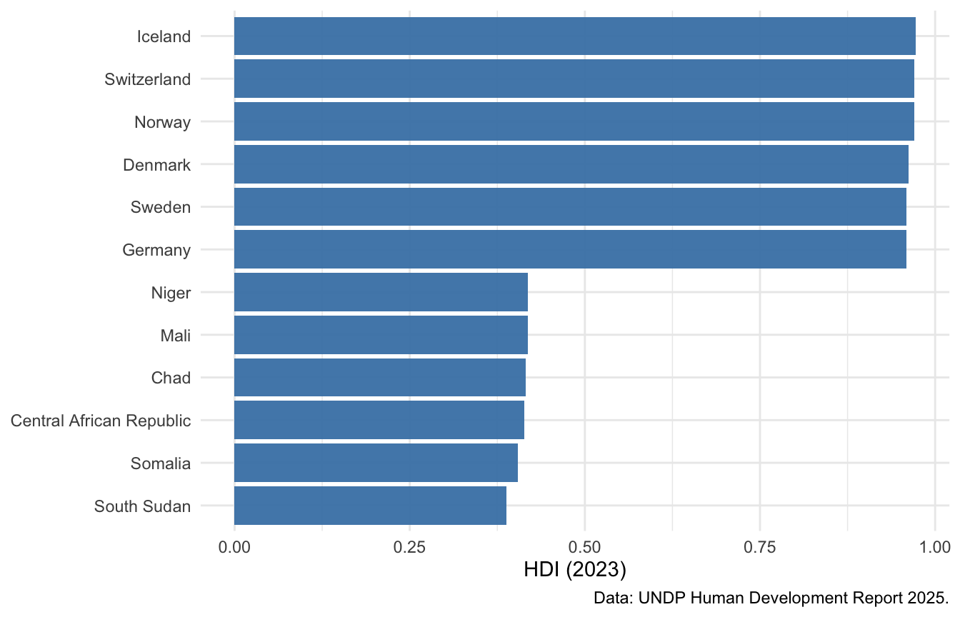
#| fig-cap: "The five highest- and five lowest-ranked countries by HDI, 2023."
#| fig-height: 4.5
#| fig-width: 7
bind_rows(
  slice_min(hdi, `Human Development Index (HDI)`, n = 5),
  slice_max(hdi, `Human Development Index (HDI)`, n = 5)
) |>
  ggplot(aes(x = reorder(Country, `Human Development Index (HDI)`),
             y = `Human Development Index (HDI)`)) +
  geom_col(fill = "steelblue", alpha = 0.95) +
  coord_flip() +
  labs(x = NULL, y = "HDI (2023)",
       caption = "Data: UNDP Human Development Report 2025.") +
  theme_minimal()
```
Now the components against each other:
```{r}
#| label: fig-hdicomponents
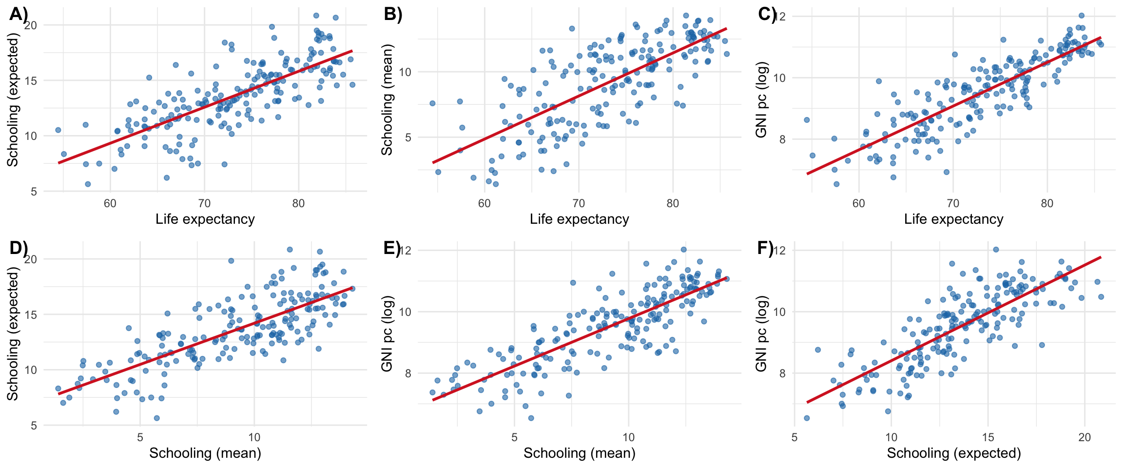
#| fig-cap: "Pairwise relationships between the HDI components. GNI per capita is shown in logs, as it enters the index."
#| fig-height: 5
#| fig-width: 12
hdi_plot <- hdi |>
  mutate(`GNI pc (log)` = log(`Gross national income (GNI) per capita`)) |>
  rename(`Schooling (expected)` = `Expected years of schooling`,
         `Schooling (mean)`     = `Mean years of schooling`,
         `Life expectancy`      = `Life expectancy at birth`)

pairs <- list(
  c("Life expectancy", "Schooling (expected)"),
  c("Life expectancy", "Schooling (mean)"),
  c("Life expectancy", "GNI pc (log)"),
  c("Schooling (mean)", "Schooling (expected)"),
  c("Schooling (mean)", "GNI pc (log)"),
  c("Schooling (expected)", "GNI pc (log)")
)

plots <- lapply(pairs, function(p) {
  ggplot(hdi_plot, aes(x = .data[[p[1]]], y = .data[[p[2]]])) +
    geom_point(alpha = 0.6, colour = "#1f77b4") +
    geom_smooth(method = "lm", se = FALSE, colour = "#d62728") +
    theme_minimal()
})

ggarrange(plotlist = plots, ncol = 3, nrow = 2,
          labels = paste0(LETTERS[1:6], ")"))
```
```{r}
#| label: tbl-hdicomponents
#| tbl-cap: "Pairwise correlations between the HDI components, ordered from strongest to weakest."
hdi |>
  select(all_of(components)) |>
  cor(use = "pairwise.complete.obs") |>
  as.data.frame() |>
  rownames_to_column("var1") |>
  pivot_longer(-var1, names_to = "var2", values_to = "correlation") |>
  filter(var1 != var2) |>
  mutate(a = pmin(var1, var2), b = pmax(var1, var2)) |>
  distinct(a, b, .keep_all = TRUE) |>
  select(`Component 1` = a, `Component 2` = b, Correlation = correlation) |>
  arrange(desc(Correlation)) |>
  kable(digits = 2) |>
  kable_styling(full_width = FALSE)
```
The correlations fall between roughly 0.64 and 0.77 — substantial, but a long
way from redundancy. The components pick up a shared underlying gradient
(countries doing well on one tend to do well on all) while each retains
considerable independent variation, which is what justifies combining them.
Two details are worth noting. The most closely related pair is the two schooling
measures, which is unsurprising since both count years of education. And the two
*weakest* pairings both involve GNI per capita — income is the component that
diverges most from the others. That is precisely the point the HDI was built to
make: how much a country produces is a genuinely imperfect guide to how long and
how educated its people's lives are.
::: {.callout-note .level-advanced}
## 🎓 MA / PhD
Correlations this high invite a natural question: why not extract the common
factor with principal components analysis and use that instead of an equally
weighted geometric mean? The statistical answer is that you could, and the first
principal component would track the HDI closely.
The reason the UNDP does not is instructive. PCA weights dimensions by how much
variance they explain, which makes the weights a property of the sample rather
than of the concept — add or remove countries and the definition of human
development shifts. Fixed equal weights are arbitrary but *stable* and
*transparent*: a reader can see what was assumed. This is a general trade-off in
index construction between statistical efficiency and interpretability, and
composite indices intended for public argument almost always choose the latter.
:::
# Directly Measured Social Indicators
Composite indices are useful for headlines and rankings. For most research
questions, a directly measured indicator is sharper: it says what it means, it
requires no aggregation assumptions, and the reader can see immediately what is
being claimed. If your question concerns child health, use child mortality — not
the HDI.
## Education
| Indicator | What it measures | WDI code |
|---|---|---|
| Adult literacy rate | Share of 15+ able to read and write | `SE.ADT.LITR.ZS` |
| Mean years of schooling | Average years completed, adults 25+ | — (UNDP) |
| Expected years of schooling | Years a child entering school can expect | — (UNDP) |
| Net enrolment ratio | Share of school-age children enrolled | `SE.PRM.NENR` |
| Primary completion rate | Share completing primary education | `SE.PRM.CMPT.ZS` |
**Sources:** UNESCO Institute for Statistics; World Bank WDI; DHS surveys.
**Miss:** all of these measure *exposure*, not *learning*. Two countries with
identical enrolment can differ enormously in what pupils actually acquire —
which is why learning-outcome measures (PISA, TIMSS, the World Bank's Learning
Poverty indicator) have become central. National averages also conceal
rural–urban and socioeconomic gaps.
## Health
| Indicator | What it measures | WDI code |
|---|---|---|
| Life expectancy at birth | Years, at current mortality rates | `SP.DYN.LE00.IN` |
| Infant mortality rate | Deaths under age 1 per 1,000 live births | `SP.DYN.IMRT.IN` |
| Under-5 mortality rate | Deaths under age 5 per 1,000 live births | `SH.DYN.MORT` |
| Maternal mortality ratio | Maternal deaths per 100,000 live births | `SH.STA.MMRT` |
| Immunisation, measles | Share of children aged 12–23 months | `SH.IMM.MEAS` |
**Sources:** WHO Global Health Observatory; World Bank WDI; UN Population
Division.
**Miss:** outcomes are shaped by much besides healthcare — nutrition,
sanitation, conflict, environment. Mental health and non-communicable disease
are poorly represented. Data quality varies sharply where vital registration is
incomplete, which is precisely where mortality is highest.
## Access to basic services
| Indicator | What it measures | WDI code |
|---|---|---|
| Access to electricity | Share of population | `EG.ELC.ACCS.ZS` |
| Safely managed drinking water | Share of population | `SH.H2O.SMDW.ZS` |
| Safely managed sanitation | Share of population | `SH.STA.SMSS.ZS` |
| Individuals using the internet | Share of population | `IT.NET.USER.ZS` |
**Sources:** WHO/UNICEF Joint Monitoring Programme; World Bank WDI; ITU.
**Miss:** access is binary and says nothing about *reliability*, *quality*, or
*affordability*. A grid connection with six hours of power a day counts as
access. Definitions of "improved" vary across contexts, and data collection
tends to have an urban bias.
## Application: the gender literacy gap
Direct indicators can be combined into something more informative than either
component alone. The **gender literacy gap** — male minus female adult literacy
— is a compact measure of unequal access to basic capabilities.^[As is common,
data are published for women and men only; other genders are generally not
recorded.]
```{r}
#| label: gender-data
literacy <- wdi_cached(
  indicators = c(
    LiteracyMale   = "SE.ADT.LITR.MA.ZS",
    LiteracyFemale = "SE.ADT.LITR.FE.ZS",
    GDPpc          = "NY.GDP.PCAP.PP.CD"
  ),
  file    = "wdi-literacy-gender.csv",
  country = "all",
  start   = 2018,
  end     = 2022,
  extra   = TRUE
)

gender_gap <- literacy |>
  filter(!is.na(region), region != "Aggregates") |>
  summarise(
    across(c(LiteracyMale, LiteracyFemale, GDPpc), \(x) mean(x, na.rm = TRUE)),
    .by = country
  ) |>
  filter(if_all(c(LiteracyMale, LiteracyFemale, GDPpc), \(x) !is.nan(x))) |>
  mutate(gap = LiteracyMale - LiteracyFemale)

nrow(gender_gap)
```
```{r}
#| label: fig-gendergap
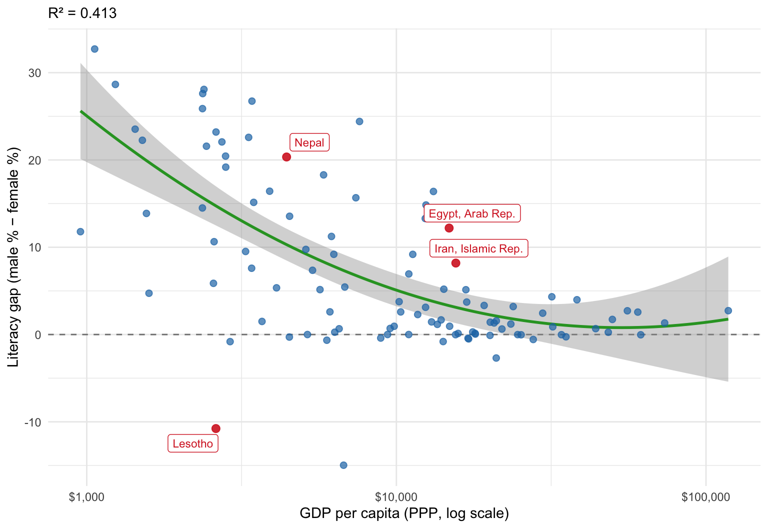
#| fig-cap: "The gender literacy gap against income per capita, averaged over 2018–2022. The fitted curve is a quadratic in log income. Positive values indicate higher male literacy."
#| fig-height: 5.5
#| fig-width: 8
highlighted <- c("Egypt, Arab Rep.", "Iran, Islamic Rep.", "Lesotho", "Nepal")

model <- lm(gap ~ poly(log(GDPpc), 2), data = gender_gap)

ggplot(gender_gap, aes(x = GDPpc, y = gap)) +
  geom_hline(yintercept = 0, linetype = "dashed", colour = "grey50") +
  geom_smooth(method = "lm", formula = y ~ poly(x, 2), se = TRUE,
              colour = "#2ca02c", linewidth = 1) +
  geom_point(data = \(d) filter(d, !country %in% highlighted),
             alpha = 0.7, colour = "#1f77b4", size = 2) +
  geom_point(data = \(d) filter(d, country %in% highlighted),
             alpha = 0.9, colour = "#d62728", size = 2.5) +
  geom_label_repel(data = \(d) filter(d, country %in% highlighted),
                   aes(label = country), colour = "#d62728", size = 3) +
  scale_x_log10(labels = scales::dollar_format()) +
  labs(
    subtitle = paste0("R² = ", round(summary(model)$r.squared, 3)),
    x = "GDP per capita (PPP, log scale)",
    y = "Literacy gap (male % − female %)"
  ) +
  theme_minimal()
```
The relationship is negative and non-linear: richer countries have smaller gaps,
with the gap closing fastest in the middle of the income range. But note what
this does *not* establish. The correlation is equally consistent with "reducing
gender inequality makes countries richer" and "richer countries find it easier
to close gender gaps", and it is consistent with both being driven by something
omitted from the picture entirely. Distinguishing these requires panel data and
an identification strategy — see
[Reasoning with DAGs](reasoning-with-dags.qmd) and
[Panel Data and Fixed Effects in R](panel-data-fixed-effects.qmd).
The outliers are often more interesting than the trend:
```{r}
#| label: tbl-outliers
#| tbl-cap: "Countries whose literacy gap departs most from the fitted relationship."
gender_gap |>
  mutate(residual = residuals(model)) |>
  filter(country %in% highlighted) |>
  select(Country = country, `GDP pc` = GDPpc,
         Male = LiteracyMale, Female = LiteracyFemale,
         Gap = gap, Residual = residual) |>
  arrange(desc(Gap)) |>
  kable(digits = c(0, 0, 1, 1, 1, 1)) |>
  kable_styling(full_width = FALSE)
```
- **Nepal** has the largest gap in the sample — over 20 percentage points — at a
low income level. Adult literacy reflects schooling received decades earlier,
so the figure records the exclusion of girls from education in the past rather
than current enrolment, which is now close to parity. Adult stock indicators
lag policy change by a generation, and this is a general caution when reading
them as evidence about present conditions.
- **Egypt and Iran** carry large gaps despite relatively high incomes. One
hypothesis is that resource exports raised income without requiring a broadly
educated workforce — consistent with the resource-curse pattern discussed in
[Income, Output, and Complexity Indicators](income-output-and-complexity-indicators.qmd).
- **Lesotho** has a strongly *negative* gap: women are markedly more literate
than men. Male labour migration to South African mines has historically pulled
boys out of school, while policy has emphasised girls' education.
These cases make the general point. A scatter plot summarises; the residuals
tell you where the summary fails, and that is usually where the research
question is.
# Summary
- The **HDI** combines health, education, and income into one number. Its
geometric aggregation encodes a substantive claim: the dimensions are
imperfect substitutes.
- The **GDI** is an HDI ratio between women and men; the **GII** uses different
dimensions and runs in the opposite direction. They are not interchangeable.
- HDI components are strongly correlated but not redundant — the composite adds
information over income alone.
- For most research questions, a **directly measured indicator** beats a
composite: it states what it means and needs no aggregation assumptions.
- Every direct indicator has a characteristic blind spot — enrolment is not
learning, access is not reliability, national averages are not distributions.
- Outliers from a fitted relationship are frequently the most informative part
of an analysis.
# References {.unnumbered}
::: {#refs}
:::