Logistic Regression for Binary Outcomes in R

Claudius Gräbner-Radkowitsch

Logistic Regression for Binary Outcomes in R

R

regression

statistics

tutorial

MA

Understand why OLS fails for binary outcomes, fit logistic regression with glm(), and translate log-odds into predicted probabilities and average marginal effects.

Author

Claudius Gräbner-Radkowitsch

Published

June 16, 2026

Modified

June 16, 2026

1 Introduction

Many outcomes of interest in economics, political science, and business are binary — a firm either exits the market or it does not; a loan is either repaid or it defaults; a voter either turns out or abstains. The familiar linear regression model runs into fundamental problems with such outcomes: it produces predicted probabilities outside [0, 1] and generates invalid standard errors.

Logistic regression solves both problems by modelling the probability of the outcome through a transformation that keeps predictions bounded between 0 and 1. The tradeoff is a more complex interpretation: instead of reading off the effect of X on Y directly, we work with log-odds, odds ratios, and — most practically — predicted probabilities.

1.1 Research question

Can we predict which firms are likely to exit the market in the next year?

1.2 Data and packages

We use the bisnode-firms dataset from Békés & Kézdi (2021). It contains roughly 17,500 Hungarian manufacturing and services firms. The outcome variable exit is a binary indicator equal to 1 if the firm closed in the following year.

Getting the data

Download bisnode-firms.csv from gabors-data-analysis.com and place it in a data/ subfolder next to this file. The dataset is distributed with the Békés & Kézdi textbook under an open data licence.

Code

library(tidyverse)
library(modelsummary)
library(marginaleffects)
library(broom)

Code

firms <- read_csv("data/bisnode-firms.csv")
glimpse(firms)

Rows: 17,506
Columns: 11
$ comp_id       <dbl> 1002029, 1011889, 1014183, 1018301, 1022796, 1035705, 10…
$ exit          <dbl> 0, 0, 0, 0, 0, 0, 0, 0, 0, 0, 0, 0, 1, 0, 0, 1, 0, 0, 0,…
$ sales_log     <dbl> 13.943477, 12.980031, 11.773208, 8.813174, 10.169549, 10…
$ employees_log <dbl> -0.78015860, 0.48317409, -0.33508429, -1.87877086, -2.48…
$ profit_margin <dbl> 0.008554417, 0.223101892, -0.018128871, -0.164738285, -0…
$ age           <dbl> 6, 20, 11, 8, 11, 1, 14, 5, 2, 4, 2, 1, 2, 4, 16, 1, 23,…
$ liquidity     <dbl> 1.69277357, 8.46944789, 24.16025018, 3.05624997, 0.90785…
$ foreign       <dbl> 0, 0, 0, 0, 0, 0, 1, 0, 0, 0, 0, 0, 0, 0, 0, 1, 0, 0, 0,…
$ female_ceo    <dbl> 0, 0, 0, 0, 0, 0, 0, 0, 0, 0, 0, 1, 1, 0, 0, 0, 0, 0, 1,…
$ industry      <dbl> 27, 55, 55, 56, 56, 56, 29, 56, 56, 27, 41, 55, 56, 28, …
$ urban         <dbl> 0, 0, 0, 0, 1, 0, 0, 0, 1, 0, 1, 1, 1, 0, 1, 0, 0, 0, 0,…

How common is firm exit in this sample?

Code

firms |>
  count(exit) |>
  mutate(share = n / sum(n))

# A tibble: 2 × 3
   exit     n  share
  <dbl> <int>  <dbl>
1     0 16294 0.931 
2     1  1212 0.0692

Exit events are relatively rare — this is typical of survival data.

2 Why OLS Fails for Binary Outcomes

2.1 The Linear Probability Model

The simplest approach is to regress the binary outcome on predictors with OLS. This is called the Linear Probability Model (LPM):

Code

lpm <- lm(exit ~ sales_log + profit_margin + employees_log, data = firms)
summary(lpm)


Call:
lm(formula = exit ~ sales_log + profit_margin + employees_log, 
    data = firms)

Residuals:
     Min       1Q   Median       3Q      Max 
-0.27563 -0.07935 -0.05414 -0.03527  1.04989 

Coefficients:
               Estimate Std. Error t value Pr(>|t|)    
(Intercept)    0.216657   0.022001   9.848  < 2e-16 ***
sales_log     -0.013902   0.001729  -8.041 9.45e-16 ***
profit_margin -0.087885   0.005908 -14.875  < 2e-16 ***
employees_log  0.005976   0.002556   2.338   0.0194 *  
---
Signif. codes:  0 '***' 0.001 '**' 0.01 '*' 0.05 '.' 0.1 ' ' 1

Residual standard error: 0.2498 on 17502 degrees of freedom
Multiple R-squared:  0.03178,   Adjusted R-squared:  0.03162 
F-statistic: 191.5 on 3 and 17502 DF,  p-value: < 2.2e-16

The LPM coefficient on profit_margin is -0.088: a one-unit increase in profit margin is associated with a -0.088 change in the probability of exit. Interpretation is direct — but does it work?

2.2 Problem 1: out-of-bounds predictions

Code

lpm_fitted <- augment(lpm, data = firms)

lpm_fitted |>
  summarise(
    min_pred     = min(.fitted),
    max_pred     = max(.fitted),
    n_below_zero = sum(.fitted < 0),
    n_above_one  = sum(.fitted > 1)
  )

# A tibble: 1 × 4
  min_pred max_pred n_below_zero n_above_one
     <dbl>    <dbl>        <int>       <int>
1  -0.0651    0.277          338           0

Some predicted “probabilities” are below 0 or above 1 — mathematically impossible.

Code

ggplot(lpm_fitted, aes(x = sales_log, y = .fitted)) +
  geom_point(alpha = 0.2, size = 0.8, color = "#2c7bb6") +
  geom_hline(yintercept = c(0, 1), linetype = "dashed", color = "firebrick") +
  annotate("label", x = max(firms$sales_log, na.rm = TRUE) - 1,
           y = -0.05, label = "Impossible: P < 0",
           color = "firebrick", size = 3) +
  labs(
    title = "LPM: fitted probabilities of firm exit",
    x = "Log sales", y = "Predicted P(exit = 1)"
  ) +
  theme_minimal()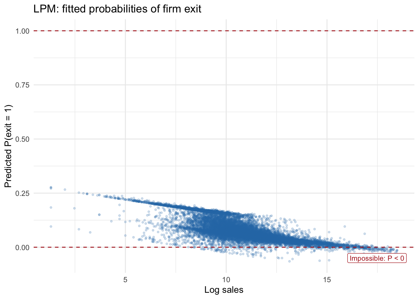

Figure 1: LPM predicted probabilities of firm exit. Values outside [0, 1] are impossible.

2.3 Problem 2: heteroskedastic errors

When Y is binary, the variance of the error term depends on X by construction:

\[\text{Var}(\varepsilon_i \mid x_i) = \hat{P}_i(1 - \hat{P}_i)\]

This violates the homoskedasticity assumption, making OLS standard errors invalid.

Note

Despite these problems, the LPM is widely used in economics, especially with panel data, because it is easy to estimate and interpret. It can serve as a useful benchmark. Always be aware of its limitations when predicted values approach 0 or 1.

3 Logistic Regression: Intuition

3.1 The logistic function

We need a function that maps any real number to a probability in [0, 1]. The logistic (sigmoid) function does exactly this:

\[\sigma(z) = \frac{e^z}{1 + e^z}\]

Code

sigma <- function(z) exp(z) / (1 + exp(z))

tibble(z = seq(-6, 6, by = 0.05)) |>
  mutate(prob = sigma(z)) |>
  ggplot(aes(z, prob)) +
  geom_line(color = "#1a9641", linewidth = 1.3) +
  geom_hline(yintercept = c(0, 0.5, 1), linetype = "dashed", color = "grey60") +
  labs(
    title = "The logistic function",
    x = "z (linear combination of predictors)",
    y = "Predicted probability"
  ) +
  theme_minimal()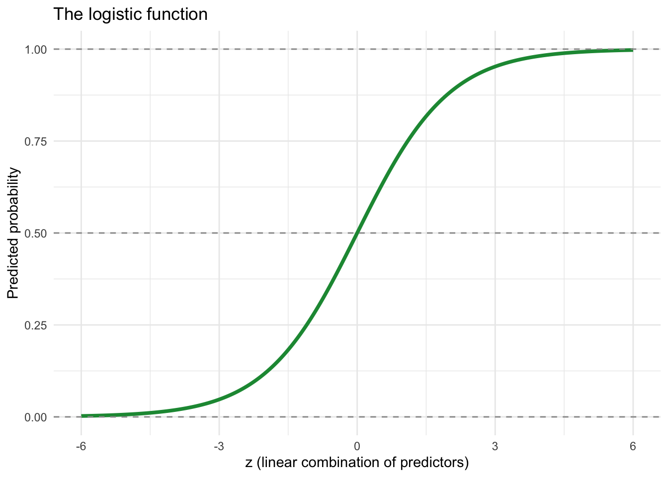

Figure 2: The logistic function maps any real number to a value in (0, 1).

The model sets \(z = \beta_0 + \beta_1 x_1 + \ldots\), so:

\[\hat{P}(\text{exit} = 1 \mid \mathbf{x}) = \frac{e^{\mathbf{X}\boldsymbol{\beta}}}{1 + e^{\mathbf{X}\boldsymbol{\beta}}}\]

3.2 The logit link

Rearranging gives the logit link — the log-odds:

\[\ln\left(\frac{P}{1-P}\right) = \beta_0 + \beta_1 x_1 + \beta_2 x_2 + \ldots\]

P(exit)	Odds	Log-odds
0.10	0.11	−2.20
0.25	0.33	−1.10
0.50	1.00	0.00
0.75	3.00	1.10
0.90	9.00	2.20

Logistic regression is estimated by maximum likelihood — not OLS. R’s glm() handles the estimation automatically.

4 Logistic Regression in R

4.1 Fitting the model

The syntax mirrors lm(). The critical addition is family = binomial:

Code

logit_model <- glm(exit ~ sales_log + profit_margin + employees_log,
                   family = binomial,
                   data = firms)

summary(logit_model)


Call:
glm(formula = exit ~ sales_log + profit_margin + employees_log, 
    family = binomial, data = firms)

Coefficients:
               Estimate Std. Error z value Pr(>|z|)    
(Intercept)   -1.048479   0.331230  -3.165  0.00155 ** 
sales_log     -0.168696   0.026067  -6.472  9.7e-11 ***
profit_margin -1.047630   0.085995 -12.183  < 2e-16 ***
employees_log  0.006127   0.043090   0.142  0.88694    
---
Signif. codes:  0 '***' 0.001 '**' 0.01 '*' 0.05 '.' 0.1 ' ' 1

(Dispersion parameter for binomial family taken to be 1)

    Null deviance: 8810.8  on 17505  degrees of freedom
Residual deviance: 8333.5  on 17502  degrees of freedom
AIC: 8341.5

Number of Fisher Scoring iterations: 6

Important

If you forget family = binomial, R silently fits a Gaussian (OLS) model on your binary outcome. Always verify your model specification.

4.2 LPM vs. logit side by side

Code

modelsummary(
  list("LPM" = lpm, "Logit" = logit_model),
  stars = TRUE,
  gof_map = c("nobs", "r.squared", "logLik", "AIC"),
  title = "Firm exit: LPM vs. logistic regression"
)

Table 1: Firm exit: LPM vs. logistic regression

Firm exit: LPM vs. logistic regression
	LPM	Logit
+ p < 0.1, * p < 0.05, p < 0.01, * p < 0.001
(Intercept)	0.217***	-1.048**
	(0.022)	(0.331)
sales_log	-0.014***	-0.169***
	(0.002)	(0.026)
profit_margin	-0.088***	-1.048***
	(0.006)	(0.086)
employees_log	0.006*	0.006
	(0.003)	(0.043)
Num.Obs.	17506	17506
R2	0.032
Log.Lik.	-556.349	-4166.748

Note: logit reports log-likelihood and AIC rather than R². These are the relevant fit statistics for maximum likelihood models.

5 Interpretation

5.1 Level 1: log-odds (raw coefficients)

Code

coef(logit_model)

  (Intercept)     sales_log profit_margin employees_log 
 -1.048478951  -0.168695919  -1.047629865   0.006126538

The coefficient on profit_margin is -1.048: a one-unit increase in profit_margin changes the log-odds of exit by that amount. The direction is clear, but the magnitude is hard to interpret intuitively.

5.2 Level 2: odds ratios

Exponentiate the coefficients:

Code

exp(coef(logit_model))

  (Intercept)     sales_log profit_margin employees_log 
    0.3504704     0.8447657     0.3507681     1.0061453

The odds ratio for profit_margin is 0.351: a one-unit increase in profit margin multiplies the odds of exit by 0.351, reducing them by 64.9%.

Code

exp(confint(logit_model))

                  2.5 %    97.5 %
(Intercept)   0.1821600 0.6674216
sales_log     0.8029502 0.8893463
profit_margin 0.2961005 0.4147961
employees_log 0.9243338 1.0944416

5.3 Level 3: predicted probabilities

Predicted probabilities are usually the most useful form for communicating results.

For the observed data:

Code

firms <- firms |>
  mutate(pred_prob = predict(logit_model, type = "response"))

firms |>
  group_by(exit) |>
  summarise(mean_pred_prob = mean(pred_prob) |> round(3))

# A tibble: 2 × 2
   exit mean_pred_prob
  <dbl>          <dbl>
1     0          0.067
2     1          0.099

Firms that actually exited had, on average, a higher predicted exit probability than survivors — the model is doing something sensible.

For specific scenarios:

Code

scenarios <- tibble(
  label         = c("Profitable, large", "Loss-making, small"),
  sales_log     = c(11, 9),
  employees_log = c(4, 2),
  profit_margin = c(0.10, -0.15)
)

scenarios |>
  mutate(
    pred_prob = predict(logit_model, newdata = scenarios, type = "response") |> round(3)
  )

# A tibble: 2 × 5
  label              sales_log employees_log profit_margin pred_prob
  <chr>                  <dbl>         <dbl>         <dbl>     <dbl>
1 Profitable, large         11             4          0.1      0.048
2 Loss-making, small         9             2         -0.15     0.083

Visualising the probability curve:

Code

grid <- tibble(
  profit_margin = seq(-0.5, 0.5, by = 0.01),
  sales_log     = mean(firms$sales_log, na.rm = TRUE),
  employees_log = mean(firms$employees_log, na.rm = TRUE)
) |>
  mutate(pred_prob = predict(logit_model, newdata = pick(everything()), type = "response"))

ggplot(grid, aes(x = profit_margin, y = pred_prob)) +
  geom_line(color = "#1a9641", linewidth = 1.2) +
  geom_hline(yintercept = c(0, 1), linetype = "dashed", color = "grey60") +
  labs(
    title = "Predicted probability of exit vs. profit margin",
    subtitle = "Other variables held at their mean",
    x = "Profit margin", y = "P(exit = 1)"
  ) +
  theme_minimal()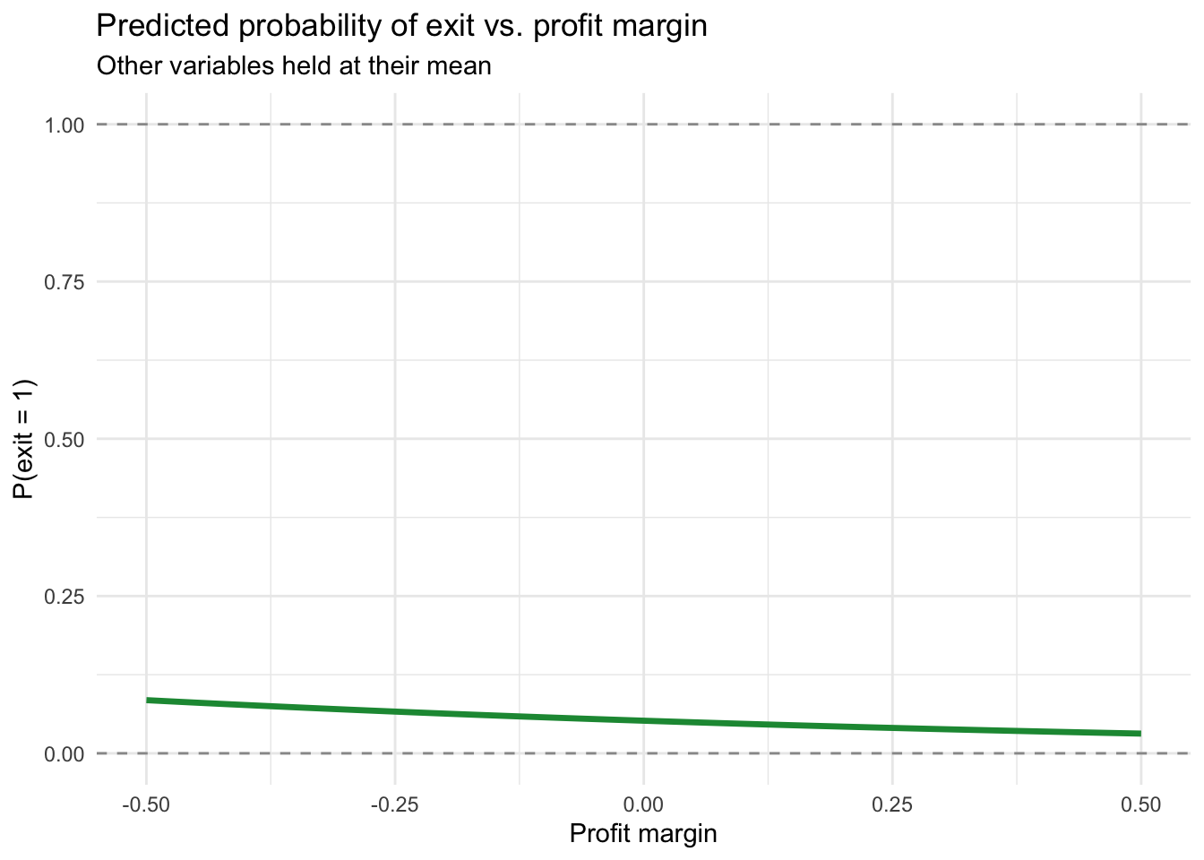

Figure 3: Predicted probability of firm exit across values of profit margin, other variables held at their mean.

5.4 Average Marginal Effects

Because logit is non-linear, the marginal effect of a predictor varies across observations. The Average Marginal Effect (AME) averages these individual marginal effects across the sample:

Code

avg_slopes(logit_model)


          Term  Estimate Std. Error       z Pr(>|z|)     S    2.5 %   97.5 %
 employees_log  0.000381    0.00268   0.142    0.887   0.2 -0.00487  0.00563
 profit_margin -0.065177    0.00546 -11.927   <0.001 106.5 -0.07589 -0.05447
 sales_log     -0.010495    0.00163  -6.445   <0.001  33.0 -0.01369 -0.00730

Type: response
Comparison: dY/dX

The AME for profit_margin directly answers: “On average across all firms, a one-unit increase in profit margin is associated with a [AME] change in the probability of exit.” This is directly comparable to the LPM coefficient.

6 Summary

Approach	Estimate	Interpretation
LPM	OLS coefficient	Change in P(Y=1) — direct but can be out of bounds
Logit — log-odds	glm coefficient	Direction clear; magnitude not intuitive
Logit — odds ratio	exp(coefficient)	Proportional change in odds
Logit — predicted prob	`predict(type="response")`	Most useful for scenarios and communication
Logit — AME	`avg_slopes()`	Average probability change; comparable to LPM

7 Practice

Apply these skills in the exercise on predicting firm exit.

8 Further Reading

Békés, G. & Kézdi, G. (2021). Data Analysis for Business, Economics, and Policy. Ch. 11. gabors-data-analysis.com
James, G., Witten, D., Hastie, T., & Tibshirani, R. (2021). An Introduction to Statistical Learning. Ch. 4. statlearning.com

Citation

BibTeX citation:

@inreference{graebner2026-logistic-regression-in-r,
  author = {Gräbner-Radkowitsch, Claudius},
  editor = {Gräbner-Radkowitsch, Claudius},
  title = {Logistic {Regression} for {Binary} {Outcomes} in {R}},
  booktitle = {Method and Inquiry},
  date = {2026-06-16},
  url = {https://euf-methodology-hub.netlify.app/resources/logistic-regression-in-r},
  langid = {en}
}

For attribution, please cite this work as:

Gräbner-Radkowitsch, Claudius. 2026. “Logistic Regression for Binary Outcomes in R.” In Method and Inquiry, edited by Claudius Gräbner-Radkowitsch. June 16. https://euf-methodology-hub.netlify.app/resources/logistic-regression-in-r.