---
title: "Measuring Inequality and Poverty"
description: "How the Lorenz curve, the Gini coefficient, top shares, and the Palma ratio describe a distribution, how absolute poverty lines and the Multidimensional Poverty Index identify deprivation, and why these measures disagree."
author: "Claudius Gräbner-Radkowitsch"
date: 2026-09-16
date-modified: 2026-09-16
image: ../assets/images/placeholder.png
learning-objectives:
- "Construct a Lorenz curve and compute a Gini coefficient from a vector of incomes"
- "Explain what the Gini, top shares, and the Palma ratio each emphasise, and why they can rank countries differently"
- "Distinguish income from wealth inequality and explain why wealth is both more concentrated and harder to measure"
- "Explain how an absolute poverty line is constructed, and what the Multidimensional Poverty Index adds to it"
categories:
- measurement
- indicators
- statistics
- R
- visualization
- tutorial
- BA
- MA
level:
- BA
- MA
content-type: tutorial
citation:
id: graebner2026-measuring-inequality-and-poverty
type: entry-encyclopedia
container-title: "Method and Inquiry"
title: "Measuring Inequality and Poverty"
editor:
- name: "Claudius Gräbner-Radkowitsch"
url: https://euf-methodology-hub.netlify.app/resources/measuring-inequality-and-poverty
---
# Introduction
Average measures such as GDP or GNI per capita say nothing about how a total is
divided. Consider two economies of ten people each. In the first, everyone earns
100 EUR. In the second, one person earns 991 EUR and the other nine earn 1 EUR
apiece. Both have a GDP of 1,000 EUR. Any indicator that cannot tell them apart
is missing something most people would consider central to development.
This page covers the two families of indicators that address this: **inequality
measures**, which describe the whole distribution, and **poverty measures**,
which focus on its bottom. They are related but not interchangeable — a country
can reduce poverty while inequality rises, and vice versa.
Both families are unusually normative. Choosing a poverty line is a statement
about what counts as a minimally acceptable life; choosing an inequality measure
is a statement about which part of the distribution matters. The general
argument for why such choices cannot be avoided is developed in
[The Theory-Ladenness of Observation](theory-ladenness-of-observation.qmd).
```{r}
#| label: setup
#| code-summary: "Packages and the caching helper"
library(WDI)
library(dplyr)
library(tidyr)
library(readr)
library(readxl)
library(purrr)
library(stringr)
library(ggplot2)
library(ggpubr)
library(kableExtra)

wdi_cached <- function(indicators, file, ...) {
  path <- file.path("data", file)
  if (!file.exists(path)) {
    message("Cache miss - downloading from the World Bank API ...")
    write_csv(WDI(indicator = indicators, ...), path)
  }
  out <- read_csv(path, show_col_types = FALSE)
  # Guard against a retired indicator code (which returns silently without its
  # column) and against a cache file written by a different query
  stopifnot(all(names(indicators) %in% names(out)))
  out
}
```
::: {.callout-important}
## Income and wealth are different things
Income is a flow (what you receive per period); wealth is a stock (what you
own). Wealth is far more concentrated than income in every country where both
have been measured, and the two behave differently: very rich households often
draw income from profits, dividends, and capital gains rather than wages, so
their *taxable income* can look modest while their wealth is enormous.
Income inequality is much easier to measure, because tax and survey systems
record income as a matter of course. Many countries — Germany among them — have
no comprehensive official statistics on the distribution of wealth at all, so
wealth figures are estimates built from partial sources. Always state which of
the two you are measuring.
:::
# Inequality Measures
## The Lorenz curve and the Gini coefficient
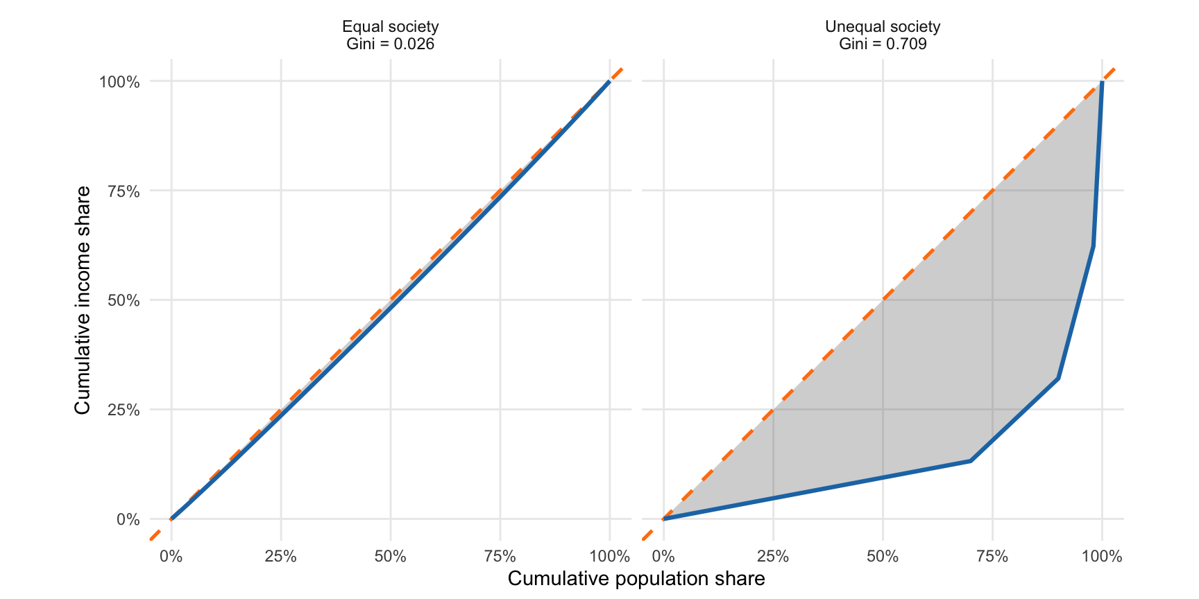
The **Lorenz curve** plots the cumulative share of total income (vertical axis)
against the cumulative share of the population, ranked from poorest to richest
(horizontal axis). Under perfect equality the poorest 30% receive exactly 30% of
income, so the "curve" is the 45-degree line. Any inequality bows the curve
below that line.
The **Gini coefficient** summarises the bow in a single number: the area between
the Lorenz curve and the line of equality, divided by the total area beneath the
line of equality. It runs from 0 (perfect equality) to 1 (one person has
everything), and is often reported as a percentage.
```{r}
#| label: fig-lorenz
#| fig-cap: "Lorenz curves for two hypothetical distributions. The shaded area between the curve and the line of equality, as a share of the whole triangle beneath that line, is the Gini coefficient."
#| fig-height: 4.5
#| fig-width: 9
#| code-summary: "Computing a Lorenz curve and Gini coefficient from scratch"
#' Lorenz curve coordinates and the Gini coefficient for a vector of incomes
lorenz_gini <- function(income) {
  sorted <- sort(income)
  n      <- length(sorted)

  # Cumulative shares, with the origin (0, 0) prepended
  pop_share    <- c(0, seq_len(n) / n)
  income_share <- c(0, cumsum(sorted) / sum(sorted))

  # Area under the Lorenz curve by the trapezoidal rule.
  # Under perfect equality that area is 1/2, so Gini = 1 - 2 * area.
  area <- sum(diff(pop_share) *
                (head(income_share, -1) + tail(income_share, -1)) / 2)

  list(pop_share = pop_share, income_share = income_share, gini = 1 - 2 * area)
}

set.seed(123)
distributions <- list(
  "Equal society"   = rep(100, 100) + rnorm(100, 0, 5),
  "Unequal society" = c(rep(10, 70), rep(50, 20), rep(200, 8), rep(1000, 2))
)

lorenz_df <- imap_dfr(distributions, function(income, label) {
  res <- lorenz_gini(pmax(income, 0))
  tibble(
    type         = paste0(label, "\nGini = ", round(res$gini, 3)),
    pop_share    = res$pop_share,
    income_share = res$income_share
  )
})

ggplot(lorenz_df, aes(x = pop_share, y = income_share)) +
  geom_ribbon(aes(ymin = income_share, ymax = pop_share),
              alpha = 0.3, fill = "grey40") +
  geom_abline(slope = 1, intercept = 0, linetype = "dashed",
              colour = "#ff7f0e", linewidth = 0.9) +
  geom_line(colour = "#1f77b4", linewidth = 1.1) +
  facet_wrap(~type) +
  coord_equal() +
  scale_x_continuous(labels = scales::percent_format(), limits = c(0, 1)) +
  scale_y_continuous(labels = scales::percent_format(), limits = c(0, 1)) +
  labs(x = "Cumulative population share", y = "Cumulative income share") +
  theme_minimal() +
  theme(panel.grid.minor = element_blank())
```
**Sources:** World Bank `SI.POV.GINI`; [WID.world](https://wid.world/); the
Luxembourg Income Study (harmonised microdata); the World Income Inequality
Database.
**Captures:** the entire distribution in one number; widely available, long time
series, internationally recognised; reasonably intuitive.
**Misses:** very different distributions can produce the same Gini, because the
measure is insensitive to *where* in the distribution inequality sits. It is
most sensitive around the middle and relatively insensitive at the extremes —
which is awkward, since the extremes are usually what the political debate is
about. It also depends heavily on survey design and coverage.
::: {.callout-warning}
## Gini coefficients are frequently not comparable
A World Bank Gini may be computed from **income** for one country and from
**consumption** for another. Consumption is distributed much more equally than
income, because rich households save a large share of what they receive. India's
World Bank Gini is around 25 — lower than Norway's — almost entirely because it
is consumption-based. Before comparing two Gini coefficients, check that they
refer to the same variable, the same unit (household vs. individual), and the
same point in the tax-and-transfer chain (pre- vs. post-redistribution).
:::
## Top and bottom shares
Share measures sidestep the aggregation problem by reporting parts of the
distribution directly: the share of total income or wealth held by the top 10%,
the top 1%, or the bottom 40%.
These are the natural measures for wealth, where survey data break down in the
upper tail and tax-based estimation is required. The methodology is actively
debated, because much wealth is unrecorded or deliberately hidden.^[On this, see
Zucman and Piketty [-@zucman2016] or Saez and Zucman [-@saez2019].]
**Captures:** what happens at the extremes, which aggregate measures average
away; changes in top-end concentration invisible to the Gini; a natural fit for
wealth data.
**Misses:** everything outside the reported segment; and they say nothing about
inequality *within* the top 10% or the bottom 40%.
## The Palma ratio
The **Palma ratio** is the income share of the top 10% divided by that of the
bottom 40%. Its motivation is an empirical regularity: across countries and over
time, the middle of the distribution (the 50th to 90th percentiles) captures
roughly half of total income, and almost all cross-country variation is in how
the remaining half is split between the top 10% and the bottom 40%. The Palma
ratio measures exactly that contested part, and some argue it is preferable to
the Gini for precisely this reason [@cobham2014].
**Captures:** the part of the distribution that actually varies; robust to
measurement error in the middle; simple to interpret ("the top tenth receives
*X* times what the bottom four tenths receive").
**Misses:** inequality within the top and bottom groups; and it relies on the
stability of the middle share, which may not hold everywhere.
## Application: income and wealth concentration compared
The [World Inequality Database](https://wid.world/) publishes top shares for
both income and wealth on a common basis, which lets us compare the two
directly. The export below was taken from the WID portal.
```{r}
#| label: wid-data
#| code-summary: "Reading and tidying the WID export"
# The WID export puts a two-line label in the `variable` column; the second
# line holds the human-readable variable name.
second_line <- function(x) map_chr(str_split(x, "\\n"), \(parts) parts[2])

wid <- read_xlsx(
  "data/wid-income-wealth-shares.xlsx",
  col_names = c("country", "variable", "percentile", "year", "value")
) |>
  mutate(
    variable = second_line(variable),
    iso3c    = countrycode::countrycode(country, "country.name", "iso3c",
                                        warn = FALSE)
  ) |>
  filter(!is.na(iso3c)) |>
  # Countries where WID reports only one of the two series
  filter(!iso3c %in% c("CHN", "GEO", "IND", "JEY", "MEX", "RUS", "ZAF")) |>
  select(-percentile) |>
  # `year` is still needed here: it is part of the key that makes each
  # country-year row unique before the two variables are spread into columns
  pivot_wider(names_from = "variable", values_from = "value") |>
  rename(wealth_top10 = `Net personal wealth`,
         income_top10 = `Pre-tax national income `) |>
  # One observation per year from 2010 to 2023; average over them
  summarise(across(c(wealth_top10, income_top10), \(x) mean(x, na.rm = TRUE)),
            .by = c("country", "iso3c"))

nrow(wid)
```
```{r}
#| label: fig-incomewealth
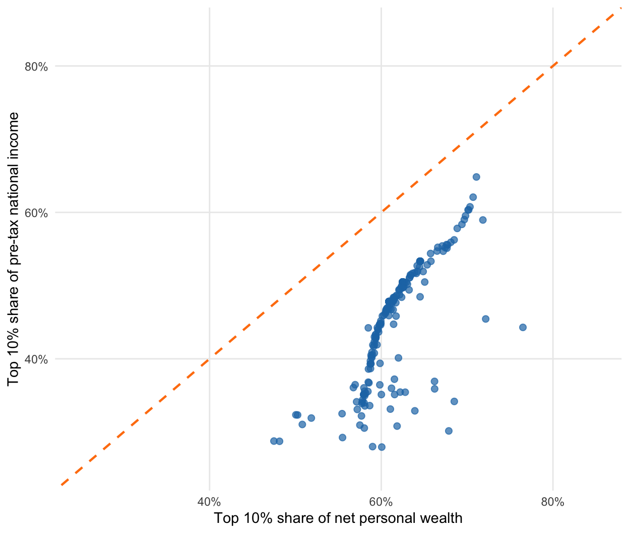
#| fig-cap: "Top 10% shares of income and of wealth, averaged over 2010–2023. The dashed line marks equal concentration of the two. Source: WID.world."
#| fig-height: 5.5
#| fig-width: 6.5
ggplot(wid, aes(x = wealth_top10, y = income_top10)) +
  geom_abline(slope = 1, intercept = 0, linetype = "dashed",
              colour = "#ff7f0e", linewidth = 0.8) +
  geom_point(size = 2, alpha = 0.7, colour = "#1f77b4") +
  scale_x_continuous(limits = c(0.25, 0.85),
                     labels = scales::percent_format(accuracy = 1)) +
  scale_y_continuous(limits = c(0.25, 0.85),
                     labels = scales::percent_format(accuracy = 1)) +
  labs(x = "Top 10% share of net personal wealth",
       y = "Top 10% share of pre-tax national income") +
  theme_minimal() +
  theme(panel.grid.minor = element_blank())
```
Two patterns stand out. First, the two are positively related: countries with
concentrated income tend to have concentrated wealth. Second, and more
strikingly, **every point lies below the diagonal** — wealth is more
concentrated than income in every country in the sample, without exception.
The methodological implication is direct. An analysis that reports only income
inequality systematically understates economic inequality, and does so in the
same direction everywhere. The choice between the two measures is not a matter
of convenience.
# Poverty Measures
## Absolute poverty lines
An absolute poverty line fixes a consumption threshold and counts the people
below it. The World Bank currently maintains three international lines, all in
2021 PPP dollars:
| Line | Purpose | WDI code |
|---|---|---|
| \$3.00 / day | Extreme poverty | `SI.POV.DDAY` |
| \$4.20 / day | Lower-middle-income standard | `SI.POV.LMIC` |
| \$8.30 / day | Upper-middle-income standard | `SI.POV.UMIC` |
The resulting **headcount ratio** is the share of the population below the line.
These thresholds are revised periodically as PPP conversion factors are
rebased — which means that poverty series are not directly comparable across
revisions, a detail often lost when the numbers are quoted.
**Captures:** an intuitive, policy-actionable threshold; long time series;
international comparability via PPP.
**Misses:** the level of the line is a value judgement, not a finding; the
binary count ignores *how far* below the line people are; PPP conversion factors
are built from national consumption baskets that may not resemble what poor
households actually buy; and World Bank estimates frequently diverge
substantially from national poverty statistics [e.g. @reddy2010].
## The Multidimensional Poverty Index
The MPI treats poverty as deprivation across several dimensions rather than a
shortfall of income. It uses ten indicators in three dimensions:
- **Health:** nutrition, child mortality
- **Education:** years of schooling, school attendance
- **Living standards:** cooking fuel, sanitation, drinking water, electricity,
housing, assets
A person counts as multidimensionally poor when deprived in at least one third
of the weighted indicators. The index then combines the *incidence* of poverty
(how many are poor) with its *intensity* (how deprived the poor are on average)
— information a headcount discards.
**Sources:** UNDP Human Development Reports; the Oxford Poverty and Human
Development Initiative (OPHI); DHS and MICS household surveys.
**Captures:** deprivations invisible to income measures; which specific
deprivations bind, which is directly useful for policy; robustness to error in
any one indicator.
**Misses:** the weighting across dimensions and the deprivation cut-offs are
judgement calls; it needs detailed household survey data, so coverage is
patchier and less frequent; and it is less comparable across very different
contexts than a monetary line.
## Application: global poverty over time
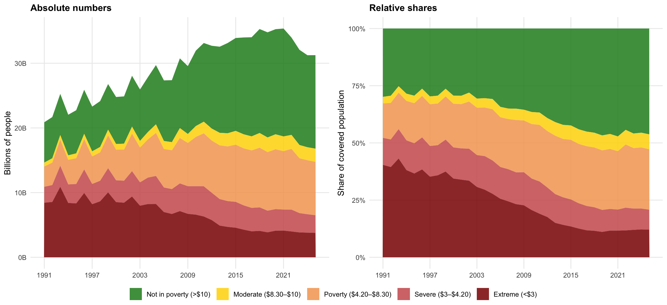
The figure below uses World Bank Poverty and Inequality Platform data as
processed and documented by [Our World in Data](https://ourworldindata.org/).
```{r}
#| label: poverty-data
#| code-summary: "Reading and reshaping the OWID poverty data"
poverty <- read_csv("data/owid-poverty-thresholds.csv",
                    show_col_types = FALSE) |>
  select(-ends_with("annotations")) |>
  pivot_longer(cols = starts_with("Number of")) |>
  mutate(name = str_remove(name, " - Income or consumption consolidated")) |>
  summarise(Total = sum(value, na.rm = TRUE), .by = c("Year", "name")) |>
  mutate(TotalPop = sum(Total), Share = Total / TotalPop, .by = "Year") |>
  filter(Year >= 1991) |>
  mutate(Category = factor(
    case_when(
      str_detect(name, "not in poverty")             ~ "Not in poverty (>$10)",
      str_detect(name, "between \\$8.30 and \\$10")  ~ "Moderate ($8.30–$10)",
      str_detect(name, "between \\$4.20 and \\$8.30")~ "Poverty ($4.20–$8.30)",
      str_detect(name, "between \\$3 and \\$4.20")   ~ "Severe ($3–$4.20)",
      str_detect(name, "\\$3 a day")                 ~ "Extreme (<$3)",
      .default = name
    ),
    levels = c("Not in poverty (>$10)", "Moderate ($8.30–$10)",
               "Poverty ($4.20–$8.30)", "Severe ($3–$4.20)", "Extreme (<$3)")
  ))
```
```{r}
#| label: fig-poverty
#| fig-cap: "People living below successive poverty thresholds, in absolute numbers and as shares of the covered population. All thresholds are contested; see the discussion below."
#| fig-height: 5.5
#| fig-width: 12
poverty_colours <- c(
  "Extreme (<$3)"         = "#8B0000",
  "Severe ($3–$4.20)"     = "#CD5C5C",
  "Poverty ($4.20–$8.30)" = "#F4A460",
  "Moderate ($8.30–$10)"  = "#FFD700",
  "Not in poverty (>$10)" = "#228B22"
)

poverty_plot <- function(data, yvar, title, ylab, ylabels) {
  ggplot(data, aes(x = Year, y = {{ yvar }}, fill = Category)) +
    geom_area(alpha = 0.85) +
    scale_fill_manual(values = poverty_colours) +
    scale_x_continuous(breaks = seq(1991, max(data$Year), by = 6)) +
    scale_y_continuous(labels = ylabels) +
    labs(title = title, x = NULL, y = ylab, fill = NULL) +
    theme_minimal() +
    theme(plot.title = element_text(size = 12, face = "bold"),
          panel.grid.minor = element_blank(),
          legend.position = "bottom")
}

ggarrange(
  poverty_plot(poverty, Total / 1e9, "Absolute numbers",
               "Billions of people", scales::comma_format(suffix = "B")),
  poverty_plot(poverty, Share, "Relative shares",
               "Share of covered population", scales::percent_format()),
  ncol = 2, common.legend = TRUE, legend = "bottom"
)
```
The headline reading — that the share in extreme poverty has fallen sharply —
is one of the most cited findings in development economics, and also one of the
most contested. The critiques bear directly on everything above: that the \$3
line is set far below any plausible subsistence requirement, that PPP
conversions misrepresent what the poor actually face, and that measuring
progress against an extremely low threshold flatters the record of the economic
order that produced it. For accessible statements of the critique see Hickel
[-@hickel2019] and Smith [-@smith2021]; for the academic exchange, Sullivan and
Hickel [-@sullivan2023] and the reply by Rutar [-@rutar2024].
::: {.callout-tip}
## An exercise worth doing
Reproduce the right-hand panel using only the \$8.30 line rather than the \$3
line, and describe the trend in words. Then write two sentences: one defensible
summary of global poverty trends using the \$3 line, and one using the \$8.30
line. Both will be true. That is the point — and it is why the choice of
threshold has to be argued for rather than inherited.
:::
# Summary
- **Inequality** measures describe the whole distribution; **poverty** measures
describe its bottom. They can move in opposite directions.
- The **Gini** summarises the Lorenz curve in one number, but is insensitive to
*where* inequality sits, and is frequently not comparable across countries
because of income-vs-consumption and pre-vs-post-redistribution differences.
- **Top shares** and the **Palma ratio** report contested parts of the
distribution directly, and are the practical choice for wealth.
- **Wealth is more concentrated than income in every country measured**, so
income-only analyses understate inequality systematically.
- **Absolute poverty lines** are transparent and comparable but encode a
contestable threshold; the **MPI** captures non-monetary deprivation at the
cost of comparability and coverage.
- Every number here rests on a normative choice. Report the choice, and where
possible report results under more than one.
# References {.unnumbered}
::: {#refs}
:::