Causal Reasoning with DAGs

Learn to use Directed Acyclic Graphs (DAGs) to distinguish causal from associational claims, identify confounders, mediators, and colliders, and determine what to control for in a regression model.

1 Introduction

Regression tells you how Y varies with X, holding other variables constant. That is a precise and useful statement — but it is not a causal statement. Whether a regression coefficient can be interpreted as the effect of X on Y depends on a separate argument about research design, which no amount of statistical testing can substitute for.

This tutorial introduces Directed Acyclic Graphs (DAGs) as a tool for making that argument explicit. A DAG is a diagram of your assumed causal model. It makes hidden assumptions visible, shows which variables to control for (and which to avoid), and clarifies what question each model specification actually answers.

1.1 Research question

Is there a gender wage gap among US workers — and what would it take to interpret a regression coefficient as evidence of discrimination?

1.2 Data and packages

We use the CPS MORG 2014 data. See Categorical Variables and Interaction Terms for setup details; the data file morg-2014-emp.csv is from gabors-data-analysis.com.

library(tidyverse)
library(broom)
library(modelsummary)
library(patchwork)
library(flextable)
library(dagitty)
library(ggdag)

raw <- read_csv("data/morg-2014-emp.csv", show_col_types = FALSE)

cps <- raw |>
  filter(
    !is.na(earnwke), earnwke > 0,
    !is.na(uhours),  uhours  > 0,
    !is.na(occ2012), !is.na(grade92),
    !is.na(age), !is.na(sex)
  ) |>
  mutate(
    wage   = earnwke / uhours,
    female = as.integer(sex == 2),
    educ   = grade92,
    occ    = factor(occ2012)
  ) |>
  filter(wage > 0, wage < 500) |>
  select(wage, female, age, educ, occ)

2 The Identification Problem

Regression answers:

“How does Y vary with X, holding controls constant?”

This is not the same as:

“What is the effect of X on Y?”

The gap between the two is closed — or not — by an identification argument: a claim about why the variation in X that the regression exploits is plausible to treat as if it were randomly assigned.

2.1 A motivating puzzle

Consider the raw gender wage gap:

cps |>
  mutate(gender = if_else(female == 1, "Female", "Male")) |>
  group_by(gender) |>
  summarise(
    N             = n(),
    `Median wage` = median(wage) |> round(2),
    `Mean wage`   = mean(wage)   |> round(2)
  ) |>
  flextable() |> autofit() |> theme_vanilla()

gender	N	Median wage	Mean wage
Female	73,734	16.15	20.25
Male	75,572	19.62	23.87

There is a clear difference. But is it discrimination? It could be. Or it could partly reflect differences in age, education, or occupation. The three-model progression below shows how much the estimated gap depends on what we control for — and why “more controls” is not always better.

3 Three Models, Three Questions

m1 <- lm(log(wage) ~ female,                    data = cps)
m2 <- lm(log(wage) ~ female + age + educ,        data = cps)
m3 <- lm(log(wage) ~ female + age + educ + occ,  data = cps)

modelsummary(
  list(
    "Model 1: Raw gap"        = m1,
    "Model 2: + Demographics" = m2,
    "Model 3: + Occupation"   = m3
  ),
  coef_map = c(
    "female" = "Female",
    "age"    = "Age",
    "educ"   = "Education (grade92)"
  ),
  gof_omit = "AIC|BIC|Log|F|RMSE",
  stars    = TRUE,
  notes    = "Occupation dummies (Model 3) omitted from display."
)

Table 1: Three models of the gender wage gap. Outcome: log(hourly wage).

	Model 1: Raw gap	Model 2: + Demographics	Model 3: + Occupation
+ p < 0.1, * p < 0.05, ** p < 0.01, *** p < 0.001
Occupation dummies (Model 3) omitted from display.
Female	-0.164***	-0.212***	-0.138***
	(0.003)	(0.003)	(0.003)
Age		0.012***	0.009***
		(0.000)	(0.000)
Education (grade92)		0.109***	0.060***
		(0.001)	(0.001)
Num.Obs.	149306	149306	149306
R2	0.016	0.271	0.384
R2 Adj.	0.016	0.271	0.382

The female coefficient changes from -0.164 (Model 1) to -0.212 (Model 2) to -0.138 (Model 3). This does not mean Model 3 is the most correct. Each model answers a different question. A DAG makes these differences explicit.

3.1 What each model claims

Model 1 — the raw gap: a pure descriptive statement. The coefficient absorbs everything that co-varies with gender: age, education, occupation, and pay discrimination.

Model 2 — controlling for demographics: age and education are plausible confounders (they affect wages and are correlated with gender). Notice that the gap grew when we added these controls: women are on average more educated than men, so their higher education was partially masking the gap in the raw data. Removing this masking reveals a larger underlying difference.

Model 3 — adding occupation: this is the key trap. If gender discrimination causes occupational sorting (women are steered toward lower-paying jobs), then occupation is a mediator — it lies on the causal path from gender to wages. Controlling for it blocks part of the very effect we are trying to measure.

4 DAG Concepts

4.1 Nodes and arrows

A DAG consists of: - Nodes — variables in the causal model - Arrows (directed edges) — representing direct causal claims (“X causes Y”) - No cycles — causes flow forward; you cannot find a path that loops back to its starting node

4.2 The three roles a variable can play

Role	Definition	What happens if you control for it?
Confounder	Common cause of X and Y	Closes a back-door path — good
Mediator	Caused by X and causes Y	Blocks the causal pathway — bad control
Collider	Caused by both X and Y	Opens a new spurious path — bad control

ImportantThe bad control problem

Controlling for a mediator does not give a better estimate of the total causal effect — it answers a different, narrower question. Controlling for a collider introduces spurious association that was not there to begin with.

5 Using dagitty and ggdag in R

dagitty lets you specify a DAG as a text string and ask computational questions about it — in particular, what adjustment sets are implied by the model. ggdag visualises the result.

5.1 Specify the wage gap DAG

gap_dag <- dagitty("dag {
  Gender -> Wage
  Gender -> Occupation
  Occupation -> Wage
}")

ggdag(gap_dag) + theme_dag()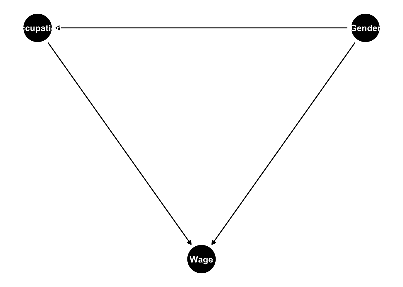

Figure 1: Gender wage gap DAG: occupation is a mediator (on the causal path from gender to wage).

5.2 Query adjustment sets

The key function is adjustmentSets(). It returns the variables you need to hold fixed to identify a stated causal effect.

Question 1: total effect of Gender on Wage

adjustmentSets(gap_dag, exposure = "Gender", outcome = "Wage")

 {}

The result is empty. Given this DAG, no controls are needed to identify the total causal effect of gender on wages. Occupation is a mediator — adding it blocks the indirect path and gives the wrong answer.

Question 2: causal effect of Occupation on Wage

adjustmentSets(gap_dag, exposure = "Occupation", outcome = "Wage")

{ Gender }

Now we must control for Gender. When the exposure changes, the adjustment set changes — even with the same DAG and the same three variables.

ImportantThe key insight

Confounder and mediator are not fixed properties of a variable. They depend on the question. Occupation is a mediator for the gender→wage question and a variable to adjust for when studying the occupation→wage question. This is why you must state your research question before deciding what to control for.

5.3 What about unobserved confounders?

gap_dag_full <- dagitty("dag {
  Gender -> Wage
  Gender -> Occupation
  Occupation -> Wage
  Background -> Wage
  Background -> Occupation
}")

adjustmentSets(gap_dag_full, exposure = "Gender", outcome = "Wage")

 {}

When we add Background (e.g., family wealth, social networks) as an unobserved confounder, the adjustment set requires controlling for it — but we cannot, because it is unobserved. This is the fundamental problem: the adjustment set tells us what we need; the data constrains what we can control for.

6 Visualising the Coefficient Path

tibble(
  model = factor(
    c("Model 1\nRaw gap", "Model 2\n+ Demographics", "Model 3\n+ Occupation"),
    levels = c("Model 1\nRaw gap", "Model 2\n+ Demographics", "Model 3\n+ Occupation")
  ),
  estimate = c(gap_m1, gap_m2, gap_m3),
  se = c(
    summary(m1)$coefficients["female", "Std. Error"],
    summary(m2)$coefficients["female", "Std. Error"],
    summary(m3)$coefficients["female", "Std. Error"]
  )
) |>
  ggplot(aes(model, estimate)) +
  geom_hline(yintercept = 0, linetype = "dashed", colour = "gray50") +
  geom_pointrange(
    aes(ymin = estimate - 1.96 * se, ymax = estimate + 1.96 * se),
    colour = "steelblue", linewidth = 0.8, size = 0.7
  ) +
  labs(
    x     = NULL,
    y     = "Coefficient on Female",
    title = "Gender wage gap across specifications",
    subtitle = "95% confidence intervals shown"
  ) +
  theme_minimal()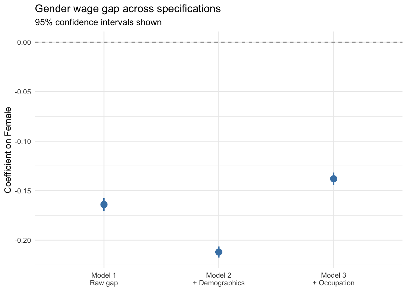

Figure 2: The female coefficient across three models. The shift from Model 2 to Model 3 is not increased precision — it is a change in the question being answered.

7 Why Observational Regression Cannot Prove Discrimination

Each of these models is a conditional association. Even Model 2 cannot rule out unobserved differences between men and women that drive both wages and correlate with gender — negotiation behaviour, network access, employer pay-setting practices.

An identification argument would need to claim: “The variation in gender I am exploiting is as good as random with respect to wages, conditional on my controls.” No observational regression on this data can credibly make that claim.

Note

This is not a failure of the data or the technique — it is a property of the question. Gender is not randomly assigned, and the labour market is not an experiment. Two strategies that can achieve identification: panel fixed effects (see Panel Data and Fixed Effects) control for all stable individual characteristics; randomised experiments such as résumé audit studies provide clean identification for narrow channels of discrimination.

8 Summary

Model	Controls	Question answered
1	None	Average raw difference — pure association
2	Age, education	Gap net of demographic composition — if no unobserved confounders
3	+ Occupation	Gap within occupation — occupation is a mediator

The coefficient changes across models not because we are getting closer to the truth, but because we are changing the question each time. A DAG makes those changes explicit and principled.

9 Practice

Apply DAG reasoning to a different substantive context in the exercise on the gender wage gap and causal reasoning.

10 Further Reading

• Pearl, J., Glymour, M., & Jewell, N. (2016). Causal Inference in Statistics: A Primer. Wiley. — The standard introduction to DAG-based causal reasoning.
• Huntington-Klein, N. (2022). The Effect: An Introduction to Research Design and Causality. Ch. 7–9. theeffectbook.net — Accessible applied treatment.
• Cunningham, S. (2021). Causal Inference: The Mixtape. mixtape.scunning.com — Free online textbook with R code.