---
title: "Income, Output, and Complexity Indicators"
description: "What GDP and GNI per capita actually measure, why the real/nominal and PPP adjustments matter, and how the Economic Complexity Index captures productive capabilities that income measures miss."
author: "Claudius Gräbner-Radkowitsch"
date: 2026-09-16
date-modified: 2026-09-16
image: ../assets/images/placeholder.png
learning-objectives:
- "Define GDP and GNI per capita and explain when the gap between them is economically informative"
- "Explain why the real/nominal and purchasing-power-parity adjustments are necessary for comparisons over time and across countries"
- "Describe what the Economic Complexity Index measures and how it differs from an income measure"
- "Assess empirically how much of the complexity–income relationship survives controlling for natural resource rents"
categories:
- measurement
- indicators
- R
- statistics
- tutorial
- BA
- MA
level:
- BA
- MA
content-type: tutorial
citation:
id: graebner2026-income-output-and-complexity-indicators
type: entry-encyclopedia
container-title: "Method and Inquiry"
title: "Income, Output, and Complexity Indicators"
editor:
- name: "Claudius Gräbner-Radkowitsch"
url: https://euf-methodology-hub.netlify.app/resources/income-output-and-complexity-indicators
---
# Introduction
This page covers the indicators that describe what an economy *produces* and
what its residents *earn*: GDP per capita, GNI per capita, and — as a measure of
the productive capabilities behind those flows — the Economic Complexity Index.
These belong together because they answer versions of the same question. GDP and
GNI ask how large the flow of output and income is. Economic complexity asks
what kind of productive structure generates that flow. Neither is a measure of
wellbeing, and the most common error in applied work is to treat them as if they
were. The companion page on
[The Theory-Ladenness of Observation](theory-ladenness-of-observation.qmd)
develops that point in general terms; here we look at what each measure does and
does not contain.
```{r}
#| label: setup
#| code-summary: "Packages and the caching helper"
library(WDI)
library(dplyr)
library(tidyr)
library(readr)
library(ggplot2)
library(ggrepel)
library(ggpubr)
library(kableExtra)

wdi_cached <- function(indicators, file, ...) {
  path <- file.path("data", file)
  if (!file.exists(path)) {
    message("Cache miss - downloading from the World Bank API ...")
    write_csv(WDI(indicator = indicators, ...), path)
  }
  out <- read_csv(path, show_col_types = FALSE)
  # Guard against a retired indicator code (which returns silently without its
  # column) and against a cache file written by a different query
  stopifnot(all(names(indicators) %in% names(out)))
  out
}
```
The `wdi_cached()` helper and the reasoning behind it are explained in
[Accessing Development Data in R](accessing-development-data-in-r.qmd).
# Gross Domestic Product
## Definition
GDP is "the market value of all final goods and services produced within a
country in a given period" [@mankiw2024, chapter 24].^[You will sometimes
encounter GDI (Gross Domestic Income), which measures the same activity from the
income side and should in principle be identical.] It aggregates cars,
haircuts, and smartphones by valuing each at its market price.
That aggregation rule has immediate consequences:
- Goods with **no market price** are largely excluded — subsistence production,
household and care work, volunteering. Where they are included at all, it is
through imputed estimates. This matters most in exactly the countries where
such activity is largest.
- Only **final** demand counts. Steel sold to a car manufacturer is not added on
top of the car.
- Only **newly produced** goods count. A new car enters GDP; the resale of a
used one does not.
## Two necessary adjustments
**Real vs. nominal.** Nominal GDP values output at each year's own prices, so it
rises when prices rise even if nothing more is produced. Real GDP holds prices
fixed at a base year. If nominal GDP doubles while all prices double, real GDP
is unchanged — and real GDP is the one that answers the question you almost
always mean to ask.
**Purchasing power parity.** Market exchange rates do not reflect what money
actually buys. 1,000 USD buys considerably more in India than in Norway, because
the Indian price level is lower. PPP conversion re-values each country's output
at a common set of prices, expressed in "international dollars". For comparisons
of living standards across countries, PPP figures are the right choice; for
questions about a country's weight in the world economy or its capacity to
import, market exchange rates are more appropriate.
::: {.callout-note}
## Choosing the right series
| Question | Series | WDI code |
|---|---|---|
| Living standards across countries | GDP pc, PPP | `NY.GDP.PCAP.PP.CD` |
| Growth within one country over time | GDP pc, constant $ | `NY.GDP.PCAP.KD` |
| Size in the world economy | GDP, current US$ | `NY.GDP.MKTP.CD` |
The Penn World Table is the standard alternative for long-run comparative work,
distinguishing expenditure-side (`rgdpe`) from output-side (`rgdpo`) real GDP.
:::
## What GDP captures and misses
**Captures:** the market value of final output; standardised across countries
through the UN System of National Accounts; long time series, back to 1960 for
most countries; frequent updates; and a robust empirical correlation with many
more fundamental welfare measures.
**Misses:** GDP was never designed as a welfare measure. It is silent on
distribution, unpriced environmental damage and resource depletion, the informal
economy and unpaid work, and the question of whether market prices track social
value at all. Its correlation with welfare measures is not a licence to treat it
as one.
# Gross National Income
GNI equals GDP plus net primary income from abroad: income earned by residents
abroad, minus income earned by non-residents domestically. GDP is about where
production *happens*; GNI is about who *receives* the income.
The World Bank's Atlas method smooths exchange-rate fluctuations using a
three-year average, and GNI per capita computed this way is the basis for the
familiar low-, lower-middle-, upper-middle- and high-income classifications.
## Application: where GDP and GNI diverge
For most countries the two are close, and the divergences are precisely the
interesting cases.
```{r}
#| label: gdp-gni-data
gdp_gni <- wdi_cached(
  indicators = c(
    GDPpc = "NY.GDP.PCAP.PP.CD",
    GNIpc = "NY.GNP.PCAP.PP.CD"
  ),
  file    = "wdi-gdp-gni.csv",
  country = c("US", "DE", "QA", "NO", "PH", "RO", "IE", "LU"),
  start   = 2000,
  end     = 2023
)

gdp_gni_avg <- gdp_gni |>
  filter(!is.na(GDPpc), !is.na(GNIpc)) |>
  summarise(across(c(GDPpc, GNIpc), mean), .by = country) |>
  mutate(
    difference     = GNIpc - GDPpc,
    difference_pct = 100 * difference / GDPpc
  )
```
```{r}
#| label: fig-gdpgni
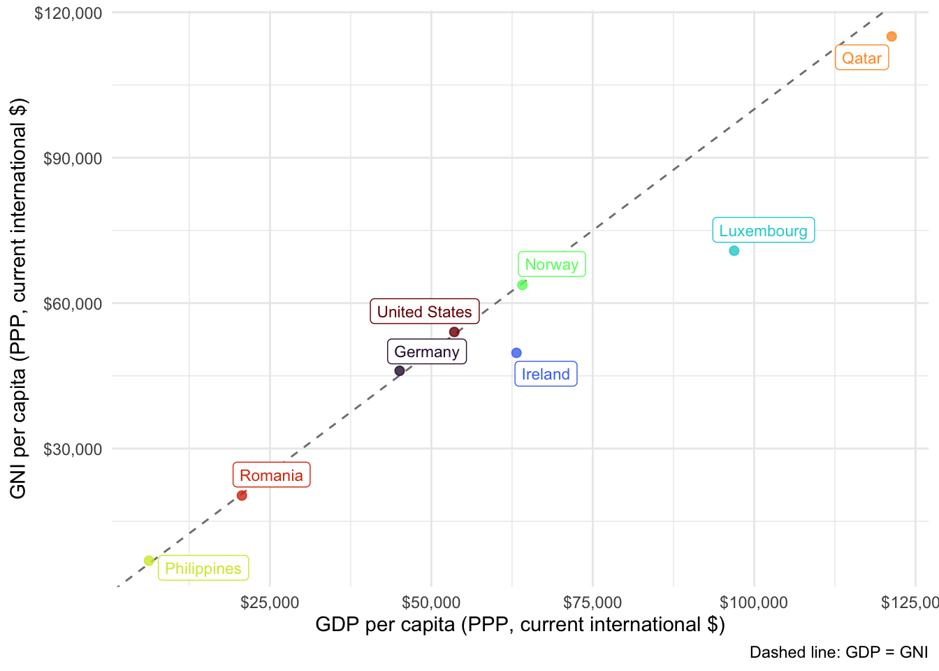
#| fig-cap: "GDP and GNI per capita (PPP), averaged over 2000–2023. Points above the dashed line are countries whose residents receive more income than is produced domestically."
#| fig-height: 5
#| fig-width: 7
ggplot(gdp_gni_avg, aes(x = GDPpc, y = GNIpc, colour = country)) +
  geom_abline(slope = 1, intercept = 0, linetype = "dashed", colour = "grey50") +
  geom_point(alpha = 0.8, size = 2) +
  geom_label_repel(aes(label = country), show.legend = FALSE, size = 3) +
  scale_colour_viridis_d(option = "H") +
  scale_x_continuous(labels = scales::dollar_format()) +
  scale_y_continuous(labels = scales::dollar_format()) +
  labs(
    x = "GDP per capita (PPP, current international $)",
    y = "GNI per capita (PPP, current international $)",
    caption = "Dashed line: GDP = GNI"
  ) +
  theme_minimal() +
  theme(legend.position = "none")
```
```{r}
#| label: tbl-gdpgni
#| tbl-cap: "Percentage difference between GNI and GDP per capita. Positive values mean GNI exceeds GDP."
gdp_gni_avg |>
  select(country, difference_pct) |>
  arrange(desc(abs(difference_pct))) |>
  rename(Country = country, `GNI − GDP (%)` = difference_pct) |>
  kable(digits = 1) |>
  kable_styling(full_width = FALSE)
```
The structural stories behind the gaps:
- **Ireland and Luxembourg**: GNI falls well short of GDP. Both host large
numbers of foreign-owned multinationals whose profits are booked domestically
and then repatriated. Irish GDP in particular is widely regarded as unusable
as a welfare indicator — Ireland's own statistical office publishes a modified
GNI (GNI\*) specifically to strip out these distortions.
- **Qatar**: GDP exceeds GNI because of income outflows to a large foreign
workforce and to foreign-owned firms in the hydrocarbon sector.
- **The Philippines**: GNI exceeds GDP, driven by remittances from a very large
overseas workforce.
The lesson is methodological rather than descriptive. GDP and GNI are close
substitutes for most purposes, but the assumption that they are interchangeable
fails exactly where a country's integration into the world economy is unusual —
which is often the case you are studying.
# Economic Complexity
## The idea
Economic complexity shifts attention from how much an economy produces to *what
it is able to produce*. The underlying claim is that development consists in
accumulating **productive capabilities** — the know-how, institutions, and
infrastructure needed to make sophisticated things — and that what a country
exports reveals which capabilities it has.^[On capabilities and their
accumulation see Aistleitner et al. [-@aistleitnerGraebnerHornykewycz2021]; on
the complexity measure itself, the [Atlas FAQ](https://atlas.hks.harvard.edu/faq)
or, at an academic level, Hidalgo [-@hidalgo2021].]
The **Economic Complexity Index (ECI)** operationalises this by looking jointly
at how *diversified* a country's export basket is and how *ubiquitous* its
products are. A country exporting many products that few others can make scores
high; a country exporting a few products that everyone makes scores low.
A closely related construct is the **product space**: a network in which
products are linked when they require similar capabilities. Peripheral products
need few capabilities; core products need many, and only complex economies make
them. The structure of the network implies that diversification is
path-dependent — countries move most easily to products adjacent to what they
already make.^[The original article remains worth reading
[@hidalgoetalProductSpace2007].]
**Sources:** the [Atlas of Economic Complexity](https://atlas.hks.harvard.edu/data-downloads)
(Harvard Growth Lab) and the [Observatory of Economic Complexity](https://oec.world/en).
**Captures:** productive capabilities invisible to GDP; a strong predictor of
subsequent growth; concrete guidance on diversification opportunities; broad
country and time coverage.
**Misses:** it is computed from *exported goods*, so services are poorly
represented and non-traded activity is invisible; it requires high-quality trade
data and so misses informal trade; the methodology is opaque to
non-specialists; and it arguably embeds a bias toward manufacturing as the route
to development.
## Application: complexity, income, and the resource curse
Complexity correlates strongly with income. But there is an obvious alternative
route to high income — exporting valuable natural resources — which requires no
complexity at all. A good test of the complexity argument therefore has to ask
how much of the relationship survives once resource wealth is accounted for.
```{r}
#| label: eci-data
#| code-summary: "Load and merge the ECI and World Bank data"
eci <- read_csv("data/eci-rankings.csv", show_col_types = FALSE) |>
  filter(year == 2021) |>
  select(iso3c = country_iso3_code, ECI = eci_hs12)

resources <- wdi_cached(
  indicators = c(
    GDPpc = "NY.GDP.PCAP.PP.CD",
    Rents = "NY.GDP.TOTL.RT.ZS"   # total natural resource rents, % of GDP
  ),
  file    = "wdi-resource-rents.csv",
  country = "all",
  start   = 2021,
  end     = 2021,
  extra   = TRUE
)

complexity <- resources |>
  filter(!is.na(region), region != "Aggregates") |>
  select(country, iso3c, GDPpc, Rents) |>
  inner_join(eci, by = "iso3c") |>
  filter(if_all(c(ECI, GDPpc, Rents), \(x) !is.na(x)))

nrow(complexity)
```
```{r}
#| label: fig-eci
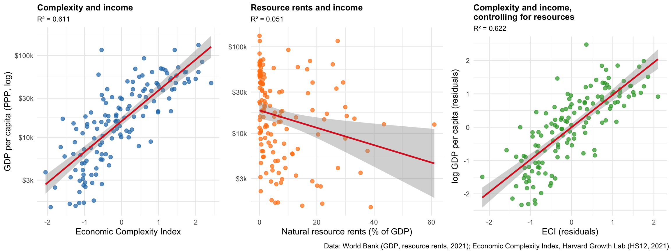
#| fig-cap: "Left: complexity and income. Centre: resource rents and income. Right: the complexity–income relationship after partialling out resource rents from both variables."
#| fig-height: 4.5
#| fig-width: 12
r2 <- function(model) round(summary(model)$r.squared, 3)

m1 <- lm(log(GDPpc) ~ ECI, data = complexity)
m2 <- lm(log(GDPpc) ~ Rents, data = complexity)

complexity <- complexity |>
  mutate(
    eci_resid = residuals(lm(ECI ~ Rents, data = complexity)),
    gdp_resid = residuals(lm(log(GDPpc) ~ Rents, data = complexity))
  )
m3 <- lm(gdp_resid ~ eci_resid, data = complexity)

base_theme <- theme_minimal() +
  theme(plot.title = element_text(size = 11, face = "bold"),
        plot.subtitle = element_text(size = 9))

p1 <- ggplot(complexity, aes(x = ECI, y = GDPpc)) +
  geom_point(alpha = 0.7, colour = "#1f77b4", size = 2) +
  geom_smooth(method = "lm", se = TRUE, colour = "#d62728", linewidth = 1) +
  scale_y_log10(labels = scales::dollar_format(scale = 0.001, suffix = "k",
                                               accuracy = 1)) +
  labs(title = "Complexity and income", subtitle = paste0("R² = ", r2(m1)),
       x = "Economic Complexity Index", y = "GDP per capita (PPP, log)") +
  base_theme

p2 <- ggplot(complexity, aes(x = Rents, y = GDPpc)) +
  geom_point(alpha = 0.7, colour = "#ff7f0e", size = 2) +
  geom_smooth(method = "lm", se = TRUE, colour = "#d62728", linewidth = 1) +
  scale_y_log10(labels = scales::dollar_format(scale = 0.001, suffix = "k",
                                               accuracy = 1)) +
  labs(title = "Resource rents and income", subtitle = paste0("R² = ", r2(m2)),
       x = "Natural resource rents (% of GDP)", y = NULL) +
  base_theme

p3 <- ggplot(complexity, aes(x = eci_resid, y = gdp_resid)) +
  geom_point(alpha = 0.7, colour = "#2ca02c", size = 2) +
  geom_smooth(method = "lm", se = TRUE, colour = "#d62728", linewidth = 1) +
  labs(title = "Complexity and income,\ncontrolling for resources",
       subtitle = paste0("R² = ", r2(m3)),
       x = "ECI (residuals)", y = "log GDP per capita (residuals)") +
  base_theme

annotate_figure(
  ggarrange(p1, p2, p3, ncol = 3),
  bottom = text_grob(
    "Data: World Bank (GDP, resource rents, 2021); Economic Complexity Index, Harvard Growth Lab (HS12, 2021).",
    size = 9, hjust = 1, x = 1)
)
```
Reading the three panels together: complexity explains a substantial share of
the cross-country variation in income; resource rents on their own explain very
little; and the complexity–income relationship is if anything slightly stronger
once resources are partialled out. Complexity is not a proxy for resource
wealth.
The countries sitting above the line in the left panel are richer than their
capability base would predict, and these are overwhelmingly resource exporters:
```{r}
#| label: tbl-outliers
#| tbl-cap: "The ten countries whose income most exceeds what their complexity predicts, ranked by the residual from the left-hand panel."
complexity |>
  mutate(residual = residuals(m1)) |>
  slice_max(residual, n = 10) |>
  select(Country = country, ECI,
         `GDP pc (PPP)` = GDPpc, `Resource rents (% GDP)` = Rents) |>
  kable(digits = c(0, 2, 0, 1)) |>
  kable_styling(full_width = FALSE)
```
```{r}
#| label: rents-comparison
complexity |>
  mutate(above_line = residuals(m1) >= sort(residuals(m1), decreasing = TRUE)[10]) |>
  summarise(mean_rents = mean(Rents), .by = above_line)
```
Their average resource rents are roughly two and a half times the sample
average. For these countries the "resource curse" literature suggests the
position is more fragile than the income figure alone implies: income without
capabilities is difficult to sustain once the resource is depleted or its price
falls.
::: {.callout-warning}
## What this analysis does not show
These are cross-sectional correlations from a single year. They are consistent
with the capability story, but they do not establish that complexity *causes*
income: rich countries can afford to build complex industries, so the causal
arrow plausibly runs both ways, and both may be driven by institutional quality
or historical circumstance. Establishing direction would require panel data and
an identification strategy — see
[Panel Data and Fixed Effects in R](panel-data-fixed-effects.qmd) and
[Reasoning with DAGs](reasoning-with-dags.qmd).
:::
# Summary
- **GDP** measures the market value of final output produced domestically. It is
well standardised and widely available, and it is not a welfare measure.
- Use **real** figures for comparisons over time and **PPP** figures for
comparisons across countries; the choice changes the answer.
- **GNI** measures income accruing to residents. Divergence from GDP flags
remittance dependence, profit repatriation, or a large foreign workforce —
which is why Ireland's and Qatar's GDP figures mislead.
- **Economic complexity** measures productive capabilities rather than income
flows, and correlates with income independently of natural resource wealth.
- All three describe production and income. None describes distribution, which
is the subject of
[Measuring Inequality and Poverty](measuring-inequality-and-poverty.qmd), or
human capabilities, covered in
[Human Development and Social Indicators](human-development-and-social-indicators.qmd).
# References {.unnumbered}
::: {#refs}
:::